For a term project in my first semester as a PhD student at the University of Michigan, in a class on landscape modeling, I wanted to investigate the relationship between socioeconomic or demographic change and land cover changes in urban areas. My intent was to produce a model sensitive to neighborhood change—particularly new development or abandonment as signaled by census measures—and to explain that change in terms of physical changes on the landscape: changes in vegetation, impervious surface, or soil cover (i.e., the VIS model) [1]. My choice of Bayesian networks was inspired by a study [2] in which they were used to determine land cover transition probabilities and, in turn, drive a cellular automata model for predicting urbanization (new urban development).
I found that while (static) Bayesian networks are very good at representing complex conditional probability distributions and reproducing static patterns, they aren't useful for predicting relatively rare events like slow and sparse land cover changes. Furthermore, the interpretation of the conditional probabilities can be somewhat subjective. Nonetheless, Bayesian networks could be a powerful tool for generalizing from a sparse dataset and may perform well on classification problems such as land cover classification.
Background
There are many motivations for studying urban environments and urban change in terms of land use or land cover changes. Studies include mitigating the impacts of urban sprawl [3], generating urban development scenarios [2], or monitoring rates of urban growth and impervious surface increase [4]. To these ends, previous studies have employed a variety of models that attempt either to predict future states of the landscape or to explain the drivers of urban change.
Some ostensibly explanatory models are not easily interpretable despite the modeler's intentions. With some cellular automata models, a failure to reproduce fine-scale patterns and accurately locate urban growth may indicate a problem with the model's structure (transition rules, namely) but identifying which parts of the structure that are at fault can be challenging as it requires many different measures of model outcomes both quantitative and qualitative [5]. Are Bayesian networks an interpretable (explanatory) and yet spatially accurate modeling approach for investigating changes in urban land cover?
Detroit is a particularly interesting case study for urban change because of its considerable economic and population decline [6]. The "greening" of Detroit—an increase in vegetation cover within the urban core due to abandonment and revegetation—is a well-documented phenomenon [7,8] that further implicates land cover change as a signal of socioeonomic and demographic change. From a modeling perspective, boom-and-bust dynamics are more challenging than constant growth and some landscape models are ill-equipped for such purposes [3].
Bayesian Networks
Bayesian networks (BNs)—also known variously as belief networks, Bayesian belief networks, Bayes nets, and causal probabilistic networks—are a relatively recent [9] tool for estimating probabilities of occurrence given sparse observations and have been demonstrated to be useful for land cover modeling. They are directed, acyclic graphs where each node is a variable and the probabilities of both "predictor" and "response" variables can be queried [10]. Nodes connected to one another imply a conditional dependence in a certain direction (hence, the graph is directed) and the links between them cannot form cycles (hence, the graph is acyclic). BNs must also exhibit the Markov property; that is, the conditional probability of any node must depend only on its immediate parents [10,11].
In general, BNs are either discrete or continuous; discrete and continuous variables are usually not mixed and software tools that support mixed types in the network are not common [10,12]. This is to facilitate calculating the joint probability distribution, which is either a multinomial distribution in the case of discrete-valued variables or a Gaussian distribution in the case of continuous values. In the case of continuous variables, the parameters are just regression coefficients. Because the nodes of a Bayesian network are linked, multivariate regression is performed to predict the distribution arising at each node in the network, providing regression coefficients for each pairwise interaction between a node and its connections [10].
Training a Bayesian network generally consists of two steps: learning the network structure and then fitting the parameters. In some studies, the network structure may be known or specified by an expert. The conditional probability tables (CPTs) for some or all of the variables might also be specified by an expert [2].
Structure learning is computationally intensive but many different algorithms are available that are all tractable on end-user hardware. The second step, fitting parameters, is generally done through a maximum likelihood approach (whereby the best fit parameters are estimated) or a Bayesian approach (whereby the posterior distribution of the parameters for a discrete distribution is estimated). The Bayesian approach is preferred as it provides more robust estimates and guarantees the conditional probability tables will be complete [10].
Bayesian Networks in R
The book Bayesian Networks in R by Nagarjan et al. [10] mentions a number of different R packages for investigating Bayesian networks.
I'll speak only about the bnlearn package [13], which I've found to be the easiest to use and yet quite robust.
I used three classes of network learning algorithms—all available in the bnlearn package for R—to investigate possible network structures and to select a stable (consistent) structure for modeling based on a random sample of my discretized training data.
Most of the algorithms I tried produced extremely dense graphs including many complete graphs (i.e., every node is connected to every other), which generally do not perform well for prediction.
Ultimately, two hybrid algorithms, General 2-Phase Restricted Maximization (RSMAX2) and Max-Min Hill Climbing (MMHC), agreed upon the same network structure.
The hybrid score and constraint-based class of algorithms is considered to produce more reliable networks than either score-based or constraint-based algorithms alone [10].
Learning Network Structure in R
The bnlearn package makes learning network structure a one-liner for any algorithm of choice.
Some algorithms have more options than others.
For instance, Incremental Association Markov Blanket (IAMB or iamb) doesn't require any parameters.
The Hill Climbing algorithm (hc) optionally allows the user to specify how many times it will randomly restart to avoid local maxima and how many times it will add, delete, or reverse arcs after a restart.
iamb(training.sample)
hc(training.sample, restart=10, perturb=5)
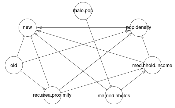
One particularly nice feature of the bnlearn package is that it has graph plotting built right in so that you can visualize the structure of the network that was learned.
mmhc.dag <- mmhc(training.sample)
plot(mmhc.dag)
We can manipulate the graphs post-hoc by setting arcs ourselves. For instance, we might want to insist that there is an arc pointing from "old" land cover to "new" land cover.
mmhc.dag <- set.arc(mmhc.dag, 'old', 'new')
Fitting Network Parameters in R
Fitting networks in bnlearn is also short and sweet.
Note that we're using a different set of training data to fit the model parameters.
The method argument is where one specifies whether to use maximum likelihood estimation (mle) or Bayesian parameter estimation (bayes); the latter is currently only implemented for discrete data sets.
fitted.network <- bn.fit(mmhc.dag, data=training.sample2, method='bayes')
An Example
The BNs were trained from high-resolution, 30-meter land cover data from 2001 and landscape measures (distance to parks and distance to roads) joined to the coarse-resolution census data for 2006. A three-folds random sample of the combined predictors was created so that the samples used to learn the network structure, score the network structure, and fit the model were disjoint. Each disjoint sample contains less than 4% of the complete dataset. The predictor variables were then aggregated to 300 meters using nearest neighbor resampling to reduce the computational complexity of prediction (classification).
Land cover classification with Bayesian networks consists of the following general steps:
- For each pixel, get the available evidence (e.g., census measures, proximities, and land cover observations).
- Obtain the posterior probability distributions given the evidence.
- Considering the "new" land cover variable, choose the outcome (e.g., land cover) from the posterior probability distribution.
I'll consider in detail each of these three steps in the following sections.
Step 1: Get the Evidence
One of the virtues of BNs is that predictions do not require a simultaneous observation of all predictor variables; even just one predictor variable can be used as evidence. Below is a striking example of how this works.
In the lower right portion of this Detroit metro area image land cover image and around the bottom and left edges there is what looks like random noise. This is an area of the scene where we have no predictor variables; it's an area consisting chiefly of the Detroit River and Windsor, Canada and, thus, was masked out in our dataset. Without any evidence to show to our model, land cover predictions are pulled from the prior distribution only. When predictions are made in areas where evidence exists, however, the posterior distribution is obtained and structure emerges.
In this step, for each pixel we want to show the network the evidence (the pixel's predictor variables or the values across all image bands).
We first need to create an independence network so that we can query our network's conditional probabilities.
This requires the gRain package.
The bnlearn package knows how to manipulate gRain data structures, provided the package is available; it provides a as.grain function to return our trained network as a gRain object.
Then, gRain compiles our network as an independence network using the junction tree algorithm.
require(gRain)

# We use the junction tree algorithm to create an independence network that we can query
prior <- compile(as.grain(fitted.network))
We call the output junction tree by the name prior as querying it will basically provide us with the prior distribution for land cover (before any evidence is shown).
# Get the prior probabilities for new land cover
querygrain(prior, nodes='new')$new
In the next step, we'll show the evidence to this independence network in order to obtain the posterior distribution.
Step 2: Show Evidence and Get the Posterior Distribution
This step is a little trickier. I had to write my own function to update the junction tree with the evidence, in particular because of the unique application to land cover classification. There's additional complexity due to the fact that our network has nodes (variables) with human-readable character strings (e.g. "med.hhold.income") but the raster layers that contain our discrete training data are integer-valued. As a result, we have to translate the raster layer class identifiers (e.g., 0, 1, 2...) into their class labels (e.g., "med.hhold.income", ...).
In the update.network function, we take in the junction tree to be modified (shown evidence) and an associative array (named list of vector in R) of the evidence (e.g., "med.hhold.income"=1, ...).
VARS <- c(...) # Some list of variable names as character strings

# A function to update the posterior probability distribution with evidence
update.network <- function (jtree, states) {
  states <- na.omit(states)

  # Do not do anything if the input data are all NA
  if (dim(states)[1] == 0) {
    return(jtree)
  }

  # Translate the raster classes [0, 1, 2, ...] into factors
  evidence <- data.frame(matrix(nrow=dim(states)[1], ncol=length(VARS)))
  names(evidence) <- VARS
  for (var in VARS) {
    evidence[,var] <- t(factors[var,][states[,var] + 1])
  }

  for (i in seq(1, dim(evidence)[1])) {
    jtree <- setEvidence(jtree, nodes=names(evidence),
                         nslist=mapply(list, evidence[i,]))
  }

  return(jtree)
}
To obtain the posterior distribution, then, looks something like this.
# Update the posterior
posterior <- update.network(prior, c(med.hhold.income=1, ...))

# Get the posterior probabilities for new land cover
querygrain(posterior, nodes='new')$new
Step 3: Predict the Outcome from the Posterior Distribution
Here, we need another convenience function; one to pick from the posterior distribution.
The choose.outcome function does this by creating a cumulative probability distribution, generating a random deviate on the uniform interval between 0 and 1, and then choosing the class that covers the interval in which the deviate is found.
For example, if there are two classes with posterior probabilities of 44% for class 0 and 56% for class 1, then a random deviate generated on [0, 0.44] will cause the pixel to be assigned to class 0 (44% of the time) while a random deviate generated on (0.44, 1.0] will cause the pixel to be assigned to class 1 (56% of the time).
# A function to choose outcomes, one at a time, with the same probability as the given posterior distribution
choose.outcome <- function (posterior) {
  posterior <- sort(posterior)

  # Sort the posterior probabilties by factors, e.g. "1=0.56,0=0.44" becomes "0=0.44,1=0.56"
  post <- numeric()
  for (i in seq.int(1, length(posterior))) {
    post[i] <- posterior[as.character(i - 1)]
  }

  # Generate a vector of probability thresholds e.g. [0.0, 0.44] for transitions to [0, 1]; upper bound of p=1.0 is implied.
  prob <- rep(0, length(post))
  for (i in seq.int(length(post) - 1, 1, by=-1)) {
    j <- length(post) - i
    prob <- prob + c(rep(0, j), post[(j-1):(length(post)-j)])
  }

  # Generate a random uniform deviate on [0, 1] to determine which factor to output
  r <- runif(1)
  for (i in seq.int(0, length(prob) - 2)) {
    if (r < prob[i + 2]) {
      return(i) # p < threshold in e.g. [0, 0.44]? Output that factor
    }
  }

  (length(prob) - 1) # p < implied upper bound of 1.0? Output last factor
}
Finally, we're ready to make some predictions, which, in this case, mean showing evidence to the network, obtaining the posterior distribution, and making a prediction by sampling from the posterior distribution.
For our land cover classification, we can use the stackApply function from the raster package to operate on a stack of raster layers, each corresponding to a predictor variable, for an efficient way of generating a vector of evidence.
require(gRain)
require(raster)

# Use the junction tree algorithm to create an independence network to query
prior <- compile(as.grain(fitted.network))

# A function to operate on each vector of predictors (vector of pixels across bands)
func <- function (r, ...) {
  choose.outcome(querygrain(update.network(prior, as.data.frame(t(r))),
                            nodes='new')$new)
}

expert.prediction <- stackApply(layers,
                                rep(1, length(names(layers))), func)
In using stackApply, we need to convert the vector of discrete raster values into a data frame with as.data.frame(t(r)) where r is the vector of raster values; we take the transpose, t(r), before turning it into a data frame so it has the right shape expected by the update.network function.
Transition Probabilities
Another neat feature of Bayesian networks is that we can easily obtain transition probabilities for our outcomes. In this case, transition probability refers to the probability that a given pixel will be assigned a certain land cover class by our model.
Recall that in the choose.outcome function we were sampling a single outcome from the posterior distribution.
To calculate transition probabilities, we instead want to assign the probability of a specific outcome for a given pixel as the value of that pixel.
This time, we use the raster calculator, calc, in the raster package to apply an arbitrary function over the pixels of our raster stack.
require(gRain)
require(raster)

# In our case, we have 3 possible outcomes
no.outcomes <- 3

# Find transition probabilities for the expert graph
trans.probs.expert <- raster::calc(layers, function (states) {
  trans <- matrix(nrow=dim(states)[1], ncol=no.outcomes)

  for (i in seq(1, dim(states)[1])) {
    # Query the network for the posterior probability of a certain "new" outcome
    trans[i,] <- querygrain(update.network(prior, as.data.frame(t(states[i,]))),
                            nodes='new')$new
  }

  return(trans)
}, forcefun=TRUE)
Below are images of the transition probabilities for the Detroit metro area land cover in 2011 as predicted from 2010 U.S. Census and landscape measures (click on each for their full resolution).
![]()
![]()
![]()
We can see that the transition probabilities all three of the predicted land cover classes—undeveloped, low development, and high development—are all fairly high but are spatially distinct. Here, "development" refers to proportion of impervious surface area as indicated by the National Land Cover Dataset (NLCD). Undeveloped areas are thought to have less than 20% impervious surface cover, low-development areas between 20% and 80%, and high-development areas more than 80%. Thus, in the "undeveloped" transition probabilities, we see very high (>/= 0.8) probabilities in the outlying suburban and exurban areas where the urban core has basically 0% chance of transitioning to undeveloped. The urban core is easily resolved in the "low development" transition probabilities and main road and highway corridors are seen in the "high development" transition probabilities, as expected.
How does our final land cover classification look? Land cover data from 2006, as the "new" or "outcome" land cover, were used to train the Bayesian network so it's no surprise the 2006 classification looks very good. The classification from 2011 is just slightly worse. The images below show the difference between the classifier's prediction and the observed NLCD land cover.

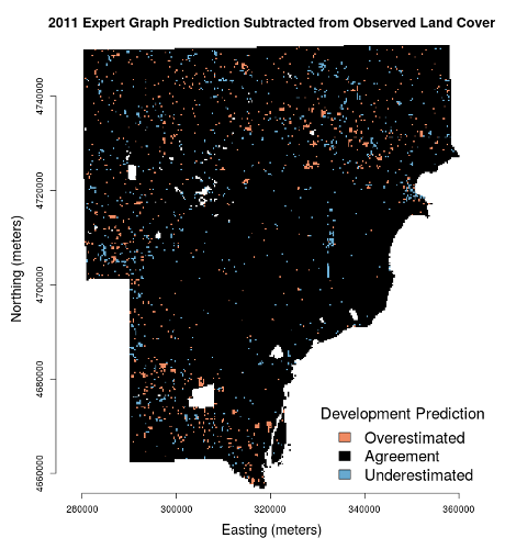
To quantify the agreement, we can use Cohen's kappa, a measure of the rank-order agreement between two sets, where the sets are the scene-wide predicted and observed land cover values, pixel for pixel. For the 2006 prediction, Cohen's kappa is 0.97—considerably high given that 1.0 would represent perfect agreement. In 2011, this agreement drops to 0.92. Different data structures are required in the training and validation process and there isn't an efficient way to remove the training pixels from the output in R. Thus, these kappas are also inflated slightly due to the inclusion of training data in the validation set, which is the entire image. However, the training data constitute less than 4% of the dataset.
Concluding Remarks
While the classification accuracies as indicated by Cohen's kappa are quite high, there are three important considerations that should mitigate our enthusiasm:
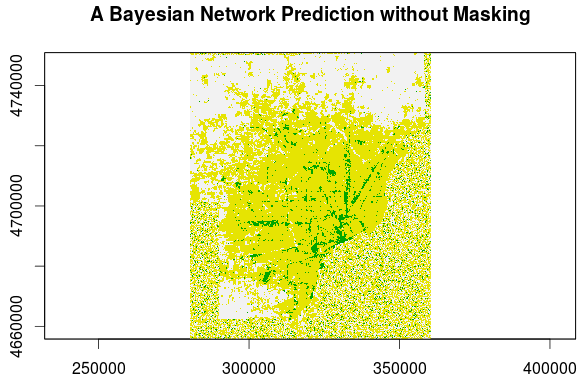
- The model completely fails to predict rare events, in this case, new urban development.
- The model included "old" land cover as a predictor, which is a considerable advantage as most pixels don't change their land cover from year-to-year.
- This classification was based in part on another classification, the NLCD "development" land cover classification.
The failure to predict rare events is related to our inclusion of "old" land cover. In a sense, there is a considerable inertia to land cover change; extant land cover rarely does change. It would be interesting to run the model again without the "old" land cover. It would also be interesting to investigate the model's performance given a remote sensing dataset rather than a previous classification. And we haven't even begun to look at the conditional probability tables! In summary, I think it's fair to say that Bayesian networks are promising for reproducing static patterns given sparse evidence and deserve attention in future land cover classification applications that are considering machine learning approaches.
References
- Ridd, M. 1995. Exploring a VIS (vegetation-impervious surface-soil) model for urban ecosystem analysis through remote sensing: comparative anatomy for cities. International Journal of Remote Sensing 16 (12):2165–2185.
- Kocabas, V., and S. Dragicevic. 2007. Enhancing a GIS Cellular Automata Model of Land Use Change: Bayesian Networks, Influence Diagrams and Causality. Transactions in GIS 11 (5):681–702.
- Jantz, C. A., S. J. Goetz, and M. K. Shelley. 2004. Using the SLEUTH urban growth model to simulate the impacts of future policy scenarios on urban land use in the Baltimore-Washington metropolitan area. Environment and Planning B: Planning and Design 31 (2):251–271.
- Sexton, J. O., X.-P. Song, C. Huang, S. Channan, M. E. Baker, and J. R. Townshend. 2013. Urban growth of the Washington, D.C.–Baltimore, MD metropolitan region from 1984 to 2010 by annual, Landsat-based estimates of impervious cover. Remote Sensing of Environment 129:42–53.
- Brown, D. G., P. H. Verburg, R. G. Pontius, and M. D. Lange. 2013. Opportunities to improve impact, integration, and evaluation of land change models. Current Opinion in Environmental Sustainability 5 (5):452–457.
- Hoalst-Pullen, N., M. W. Patterson, and J. D. Gatrell. 2011. Empty spaces: neighbourhood change and the greening of Detroit, 1975–2005. Geocarto International 26 (6):417–434.
- Emmanuel, R. 1997. Urban vegetational change as an indicator of demographic trends in cities: the case of Detroit. Environment and Planning B: Planning and Design 24:415–426.
- Ryznar, R. M., and T. W. Wagner. 2001. Using Remotely Sensed Imagery to Detect Urban Change: Viewing Detroit from Space. Journal of the American Planning Association 67 (3):327–336.
- Pearl, J. 1985. Bayesian networks: A model of self-activated memory for evidential reasoning. In Seventh Annual Conference of the Cognitive Science Society.
- Nagarajan, R., M. Scutari, and S. Lebre. 2013. Bayesian Networks in R. New York, New York, USA: Springer.
- Charniak, E. 1991. Bayesian Networks without Tears. AI Magazine 12 (4).
- Uusitalo, L. 2007. Advantages and challenges of Bayesian networks in environmental modelling. Ecological Modelling 203 (3-4):312–318.
- Scutari, M. 2014. bnlearn - an R package for Bayesian network learning and inference. http://www.bnlearn.com