Urban environments are heterogeneous at relatively small scales and composed of a variety of land covers, chiefly including impervious surface, green vegetation (e.g., the urban canopy), and soil. Ridd (1995) demonstrated that urban land cover was dominated by these three types, summarized as the Vegetation-Impervious-Soil (VIS) model. The model suffers due to the vagaries of any urban land cover analysis: There are multiple subtypes of each land cover with different spectral characteristics (e.g., multiple impervious surface colors, different vegetation species) and impervious surface and soil are easily confused. Nonetheless, the VIS model is still useful and remains one of the most popular, widely applicable descriptions of urban land cover composition (e.g., Phinn et al. 2002; Small 2003; Kärdi 2007).
How can we identify VIS areas with remote sensing? If we can spectrally separate vegetation, impervious surface, and soil then we may be able classify a multispectral image on that basis. At the resolution of many earth-observing sensors (e.g., Landsat MSS, Landsat TM/ETM+, SPOT), however, the ground sample distance of a pixel is much larger than the minimum mapping unit of urban areas (Small 2003). That is, many if not most of the pixels in the scene are mixtures of two or more VIS components (e.g., vegetation and impervious surface co-located in a suburban development). Linear spectral mixture analysis (LSMA) is one way of modeling land cover mixtures to estimate the abundance of VIS components on the ground. LSMA can be challenging and time-consuming to implement, however.
As an alternative, some investigators have introduced land cover indices based on band ratios that attempt to capture the spatial variability in the three VIS components. The Normalized Difference Vegetation Index (NDVI) is probably the most popular example of a land cover index based on band ratios. NDVI wasn't expressly intended for use in urban areas but many more recent developments are. These include the Biophysical Composition Index (BCI; Deng and Wu 2012), the Normalized Difference Impervious Surface Index (NDISI; Xu 2010), the Modified NDISI (MNDISI; Liu et al. 2013), and the Ratio Normalized Difference Soil Index (RNDSI; Deng et al. 2015).
Here, I'll focus on only the BCI as it is based on the well-known tasseled cap transformation (Kauth and Thomas 1976), a coordinate transformation that is similar to principal components analysis (PCA) and similar dimension reduction techniques that I've used in spectral mixture analysis. I'll present an overview of BCI, the tasseled cap, and examples of implementing both in Python.
The Tasseled Cap Transformation
Calculating the BCI requires the tasseled cap transformation, a coordinate transformation of multispectral remote sensing data. Tasseled cap was originally developed for Landsat MSS 4-band data. As such, the tasseled cap transformation, as initially described, produced just two principal components termed "brightness" and "greenness." These principal components have physical meanings, however, and Kauth and Thomas (1976) and later investigators (Crist and Kauth 1986) demonstrated how it could be used to track changes in the phenology of vegetation, particularly agriculture.
The lifecycle of agricultural land proceeds from bare soil to emerging vegetation, to mature green vegetation that completely covers the visible ground area, to senescent yellow vegetation, and finally to bare soil again (Kauth and Thomas 1976, Figure 2). This lifecycle is accompanied by changes in spectral reflectance of the agricultural land and if pixels in each stage are plotted in multispectral feature space, they trace a line through the space that corresponds to the temporal evolution of the landscape. They also clearly fall into separate regions. If a new coordinate system is aligned with these features it is possible to compress over 95% of the information stored in four (4) MSS bands into just two bands ("brightness" and "greenness"). The tasseled cap's name is derived from its appearance in feature space once the coordinate transformation is performed.
The tasseled cap transformation has a compact mathematical notation but requires a table of rotation coefficients (see Kauth and Thomas 1976) for the \(p\times p\) rotation matrix, \(R\). A \(p \times n\) vector \(x\) of multispectral data (comprised of \(p\) spectral bands across \(n\) pixels) is transformed to a \(u\) vector by means of the following rotation, where \(e\) is an optional translation that can be used to avoid negative values in the transformed data:
Kauth and Thomas provided the coefficients in \(R\) for the Landsat MSS sensor in their 1976 paper that introduced the transformation. Those Landsat MSS coefficients were based on MSS data provided in counts. Since then, others have presented versions of the tasseled cap transformation for other platforms and sensors such as Landsat TM surface reflectance (Crist and Cicone 1984), Landsat ETM+ top-of-atmosphere (TOA) reflectance (Huang et al. 2002), MODIS (Lobser et al. 2007), WorldView-2 (Yarbrough et al. 2014), and Landsat 8 TOA reflectance (Baig et al. 2014).
Below is a simple Python implementation of the tasseled cap transformation, without support for the optional translation. The coefficients are those for Landsat TM surface reflectance (via Crist and Cicone 1984) but could be replaced with the relevant coefficients for any other sensor data. Landsat surface reflectance data can be obtained easily from the USGS EROS Science Processing Architecture (ESPA). The function accepts a Landsat TM surface reflectance raster as either a GDAL data source or a \(p\times m\times n\) NumPy array where \(p\) is the number of bands, and \(m, n\) refer to the number of rows and columens, respectively.
def tasseled_cap_tm(rast, reflectance=True):
    '''
    Applies the Tasseled Cap transformation for TM data. Assumes that the TM
    data are TM reflectance data (i.e., Landsat Surface Reflectance). The
    coefficients for reflectance factor data are taken from Crist (1985) in
    Remote Sensing of Environment 17:302.
    '''
    if reflectance:
        # Reflectance factor coefficients for TM bands 1-5 and 7; they are
        #   entered here in tabular form so they are already transposed with
        #   respect to the form suggested by Kauth and Thomas (1976)
        r = np.array([
            ( 0.2043, 0.4158, 0.5524, 0.5741, 0.3124, 0.2303),
            (-0.1603,-0.2819,-0.4934, 0.7940,-0.0002,-0.1446),
            ( 0.0315, 0.2021, 0.3102, 0.1594,-0.6806,-0.6109),
            (-0.2117,-0.0284, 0.1302,-0.1007, 0.6529,-0.7078),
            (-0.8669,-0.1835, 0.3856, 0.0408,-0.1132, 0.2272),
            ( 0.3677,-0.8200, 0.4354, 0.0518,-0.0066,-0.0104)
        ], dtype=np.float32)

    else:
        raise NotImplemented('Only support for Landsat TM reflectance has been implemented')

    shp = rast.shape

    # Can accept either a gdal.Dataset or numpy.array instance
    if not isinstance(rast, np.ndarray):
        x = rast.ReadAsArray().reshape(shp[0], shp[1]*shp[2])

    else:
        x = rast.reshape(shp[0], shp[1]*shp[2])

    return np.dot(r, x).reshape(shp)
When I first implemented this in Python, I naturally wanted to check to make sure I had it right. So, I plotted the first three tasseled cap (TC) components, Brightness, Greenness, and Wetness, in feature space. We can compare these images to the figures in Kauth and Thomas (1976) or Crist and Cicone (1984) to make sure we're on the right track.
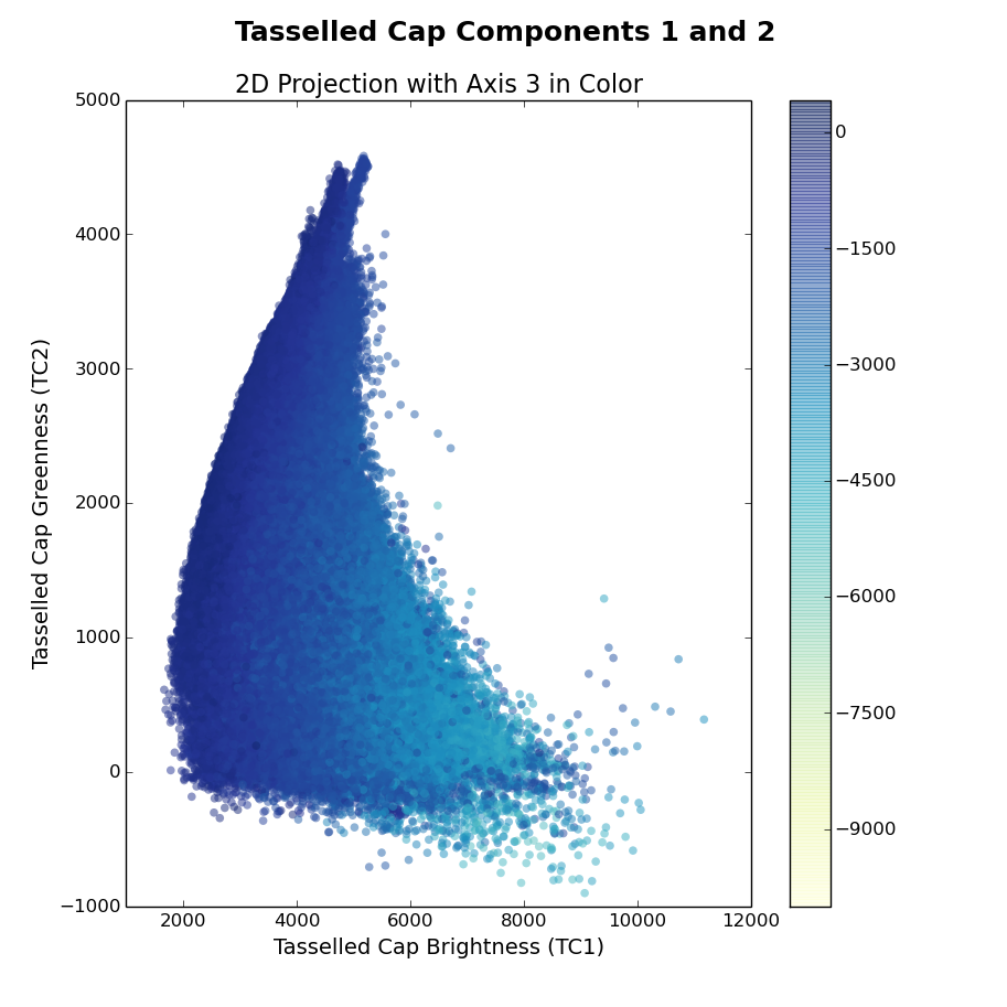
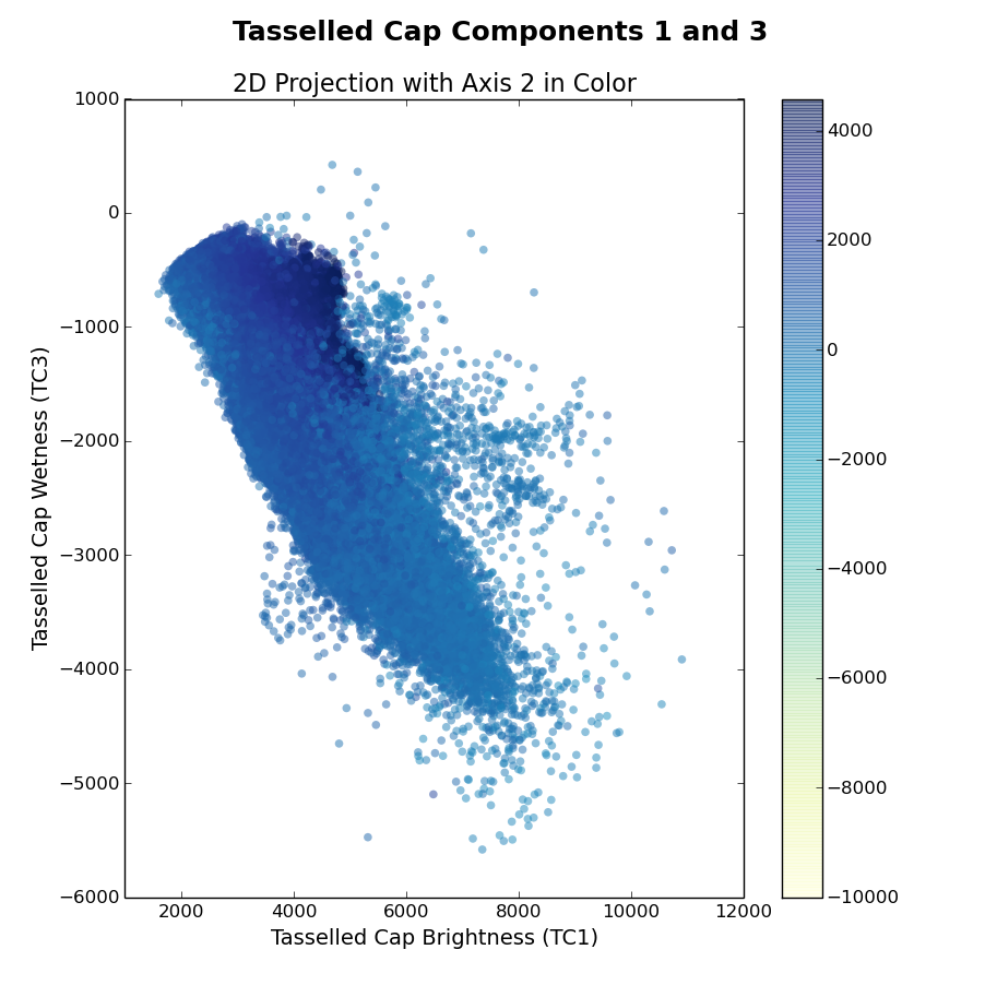
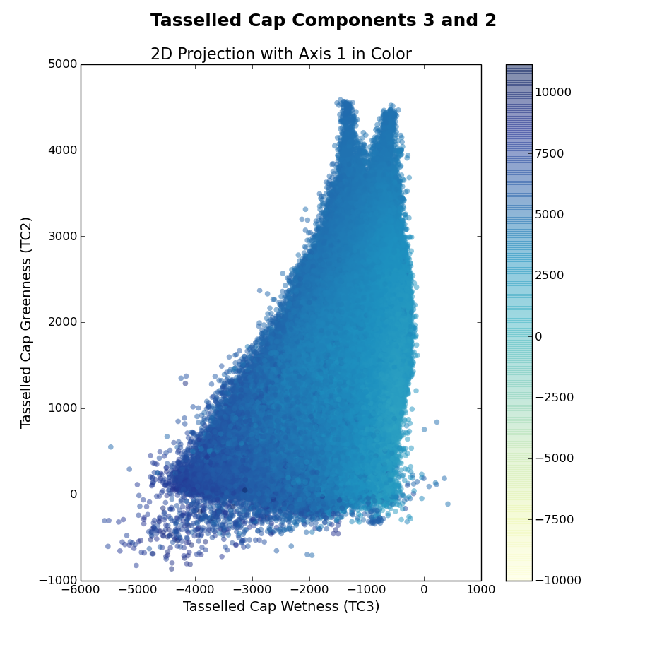
The left image shows the Brightness-Greenness plane, where we can see the eponymous tasseled cap itself. The middle image is Brightness-Wetness plane and while it doesn't look exactly like the figure in Crist and Cicone (1984), it's not wildly different. The right image is the so-called "transition zone" view; the Wetness-Grenness plane. The transition zone view looks correct although it has a very interesting fork at the top part of volume.
The Biophysical Composition Index (BCI)
Now that I can calculate the tasseled cap components I can also calculate the BCI. The BCI was developed as a one-dimensional measure of urban land cover composition based on the observation that the average values of the Brightness and Wetness tasseled cap components are much higher than the average value of the Greenness component. Deng and Wu (2012) proposed a normalized difference approach that compresses the information in the first three tasseled cap components into a measure defined on the interval \([-1, 1]\). It is defined:
Where \(H, V, L\) refer to the normalized first three tasseled cap components, \(TC1, TC2, TC3\), normalized such that:
Below is a simple Python implementation of the BCI.
def biophysical_composition_index(rast, nodata=-9999):
    '''
    Calculates the biophysical composition index (BCI) of Deng and Wu (2012)
    in Remote Sensing of Environment 127. The input raster is expected to be
    a tasseled cap-transformed raster. The NoData value is assumed to be
    negative (could never be the maximum value in a band).
    '''
    shp = rast.shape

    # Can accept either a gdal.Dataset or numpy.array instance
    if not isinstance(rast, np.ndarray):
        x = rast.ReadAsArray().reshape(shp[0], shp[1]*shp[2])

    else:
        x = rast.reshape(shp[0], shp[1]*shp[2])

    unit = np.ones((1, shp[1] * shp[2]))

    stack = []
    for i in range(0, 3):
        # Calculate the minimum values after excluding NoData values
        tcmin = np.setdiff1d(x[i, ...].ravel(), np.array([nodata])).min()

        # Calculate the normalized TC component TC_i for i in {1, 2, 3}
        stack.append(np.divide(np.subtract(x[i, ...], unit * tcmin),
            unit * (x[i, ...].max() - tcmin)))

    # Unpack the High-albedo, Vegetation, and Low-albedo components
    h, v, l = stack

    return np.divide(
        np.subtract(np.divide(np.add(h, l), unit * 2), v),
        np.add(np.divide(np.add(h, l), unit * 2), v))\
        .reshape((1, shp[1], shp[2]))
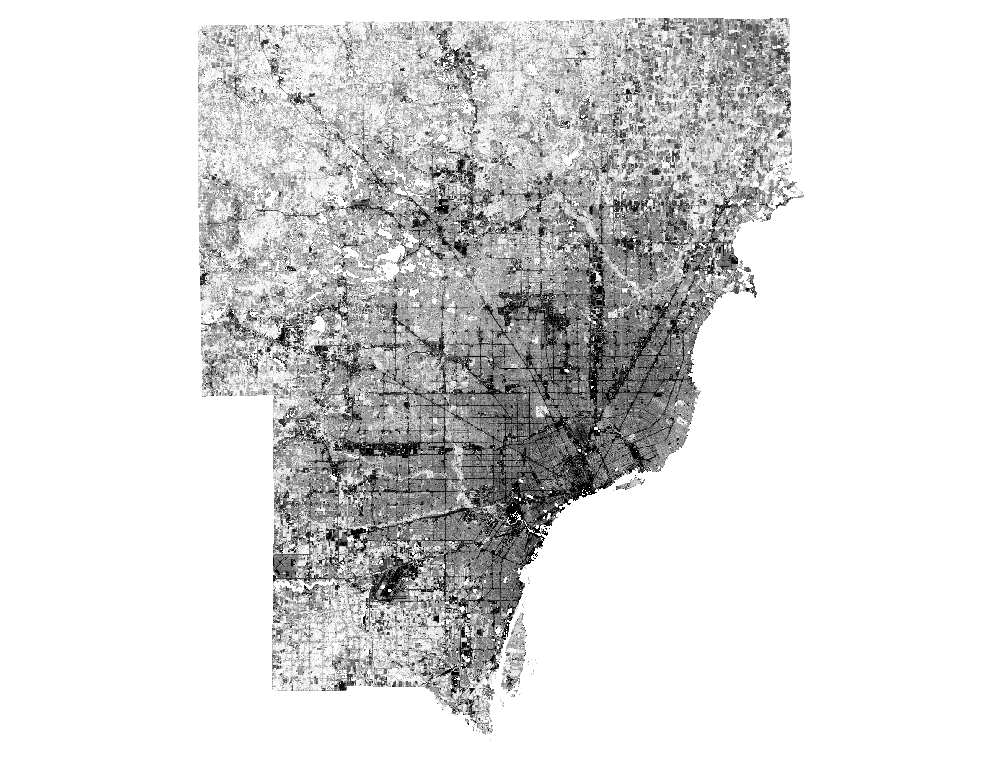
Deng and Wu found significant positive correlation between the BCI and impervious surface, significant negative correlation between the BCI and vegetation cover. I can confirm that BCI seems to be an excellent indicator of these land covers, as it is positively correlated with the National Land Cover Dataset (NLCD) impervious surface fraction. The 2001 NLCD impervious layer (left) and a BCI image calculated from a July 2002 Landsat TM image (right) are shown below; the Pearson's correlation coefficient between the datasets is \(r=0.624\).

I also compared the BCI to measures of vegetation, impervious surface, and soil derived through spectral mixture analysis of a 1998 Landsat TM image. The correlation matrix is below and indicates that these independently derived land covers are strongly correlated with the BCI. In this case, however, the soil fraction from spectral mixture analysis is likely a mixed endmember with non-photosynthetic vegetation and therefore cannot be readily interpreted in this context.
Pearson's Correlation Coefficients (r)

              BCI   Veg.    Imp.   Soil
----------  ----- ------  ------  -----
BCI         1.000 -0.877   0.838  0.538
Vegetation         1.000  -0.724 -0.810
Impervious                 1.000  0.182
Soil                              1.000
References
- Ridd, M. 1995. Exploring a VIS (vegetation-impervious surface-soil) model for urban ecosystem analysis through remote sensing: comparative anatomy for cities. International Journal of Remote Sensing 16 (12):2165–2185.
- Phinn, S., M. Stanford, P. Scarth, A. T. Murray, and P. Shyy. 2002. Monitoring the composition of urban environments based on the vegetation-impervious surface-soil (VIS) model by subpixel analysis techniques. International Journal of Remote Sensing 23 (20):4131–4153.
- Small, C. 2003. High spatial resolution spectral mixture analysis of urban reflectance. Remote Sensing of Environment 88 (1-2):170–186.
- Kärdi, T. 2007. Remote sensing of urban areas: Linear spectral unmixing of Landsat Thematic Mapper images acquired over Tartu (Estonia). Proc. Estonian Acad. Sci. Biol. Ecol 56 (1):19–32.
- Deng, C., and C. Wu. 2012. BCI: A biophysical composition index for remote sensing of urban environments. Remote Sensing of Environment 127:247–259.
- Xu, H. 2010. Analysis of Impervious Surface and its Impact on Urban Heat Environment using the Normalized Difference Impervious Surface Index (NDISI). Photogrammetric Engineering & Remote Sensing 76 (5):557–565.
- Liu, C., Z. Shao, M. Chen, and H. Luo. 2013. MNDISI: A multi-source composition index for impervious surface area estimation at the individual city scale. Remote Sensing Letters 4 (8):803–812.
- Deng, Y., C. Wu, M. Li, and R. Chen. 2015. RNDSI: A ratio normalized difference soil index for remote sensing of urban/suburban environments. International Journal of Applied Earth Observation and Geoinformation 39:40–48.
- Kauth, R. J., and G. S. Thomas. 1976. The tasseled cap - A graphic description of the spectral-temporal development of agricultural crops as seen by Landsat. In Proceedings of the Symposium on Machine Processing of Remotely Sensed Data, West Lafayette, Indiana, U.S.A, 29 June-1 July 1976, 41–51.
- Crist, E. P., and R. J. Kauth. 1986. The Tasseled Cap de-mystified. Photogrammetric Engineering and Remote Sensing 52 (1):81–86.
- Crist, E. P., and R. C. Cicone. 1984. A Physically-Based Transformation of Thematic Mapper Data---The TM Tasseled Cap. IEEE Transactions on Geoscience and Remote Sensing GE-22 (3):256–263.
- Huang, C., B. Wylie, L. Yang, C. Homer, and G. Zylstra. 2002. Derivation of a tasseled cap transformation based on Landsat 7 at-satellite reflectance. International Journal of Remote Sensing 23 (8):1741–1748.
- Lobser, S. E., and W. B. Cohen. 2007. MODIS tasseled cap: land cover characteristics expressed through transformed MODIS data. International Journal of Remote Sensing 28 (22):5079–5101.
- Yarbrough, L. D., K. Navulur, and R. Ravi. 2014. Presentation of the Kauth–Thomas transform for WorldView-2 reflectance data. Remote Sensing Letters 5 (2):131–138.
- Baig, M. H. A., L. Zhang, T. Shuai, and Q. Tong. 2014. Derivation of a tasseled cap transformation based on Landsat 8 at-satellite reflectance. Remote Sensing Letters 5 (5):423–431.