I recently found myself in need of a comprehensive water body mask I could generate from and apply to Landsat TM/ETM+ images. Based on my past experience and the available literature (e.g., Frazier et al. 2000), I knew that any solution was best sourced from Landsat's thermal bands. I wasn't entirely sure what to expect from a solution based only on spectral data but Frazier et al. (2000) presented a very robust solution using only density slicing of Landast TM Band 5 (1.55-1.75 um).
I decided I would test density slicing and compare the results to a simple supervised classification, just as Frazier et al. (2000) had done. They selected a maximum likelihood classifier; I selected a naive Bayes classifier. The study area is the Oakland county, Michigan subset of a Landsat 5 image from July, 1999. Oakland county has several small and mid-size lakes throughout its extent that make for a compelling example. The examples below require, among other tools, the GDAL and OGR command line utilities.
Data Preparation
Supervised classification requires examples of the classes we wish to identify; in this case, water bodies and non-water areas. Example areas of water and non-water were generated in two different ways:
- In one iteration, the water areas were generated directly from hydrology data provided by the Michigan Geographic Data Library (MiGDL).
- In the second iteration, I prepared examples of water and non-water areas myself in random samples from the study area.
For the second part, I wrote a previous article on how to generate sampling areas on the same grid as a Landsat image; see that article for details. Here, I proceed as if the human-produced training data are already prepared.
Projection Issues
Use of MiGDL data can be frustrating because the data are stored in the Michigan State Plane projection. In clipping the lake and stream data to Oakland county, for instance, I had to ensure my clipping features were in the same projection. I re-projected the clipped data to UTM 17N (WGS84) afterwards.
MICHIGAN_GEOREF='PROJCS["NAD_1983_Michigan_GeoRef_Meters",GEOGCS["GCS_North_American_1983",DATUM["North_American_Datum_1983",SPHEROID["GRS_1980",6378137,298.257222101]],PRIMEM["Greenwich",0],UNIT["Degree",0.017453292519943295]],PROJECTION["Hotine_Oblique_Mercator"],PARAMETER["False_Easting",2546731.496],PARAMETER["False_Northing",-4354009.816],PARAMETER["Scale_Factor",0.9996],PARAMETER["Azimuth",337.255555555556],PARAMETER["Longitude_Of_Center",-86],PARAMETER["Latitude_Of_Center",45.30916666666666],UNIT["Meter",1],AUTHORITY["EPSG","102123"]]'

# Create clipping features in Michigan GeoRef
ogr2ogr clip_features.shp Oakland_county.shp -t_srs $MICHIGAN_GEOREF

# Perform the clip
ogr2ogr -f "ESRI Shapefile" -s_srs $MICHIGAN_GEOREF\
 hydropoly_miv14a_clip.shp hydropoly_miv14a.shp\
 -t_srs "EPSG:32617" -clipsrc clip_features.shp
Cleaning the Hydrology Exemplar Data
After reprojeciton, the lake and stream areas delineated in the MiGDL dataset were filtered, discarding water bodies smaller than 20 acres, which might be ephemeral.
ogr2ogr -where "ACRES >= 20" hydropoly_miv14a_clip_gte_20ac.shp hydropoly_miv14a_clip.shp
Next, the filtered water bodies were shrunk in size by diminishing their outward edges by 90 meters---a reverse buffering. This is to account for a lack of spatial fit between the MiGDL data and the Landsat data and also eliminates uncertainty in our water area model due to nearshore vegetation cover.
ogr2ogr hydropoly_miv14a_clip_gte_20ac_shrink_90m.shp hydropoly_miv14a_clip_gte_20ac.shp -dialect sqlite -sql "SELECT GID, ACRES, SQKM, ST_Buffer(Geometry, -90) FROM hydropoly_miv14a_clip_gte_20ac"
The final step in preparing known examples of water cover is to rasterize the layer of known water bodies and clip it to the area of analysis.
For this, I used my own gdal_extent.py utility and the gdal_rasterize command line utility.
In this iteration, all Landsat pixels not intersected by the water area examples are considered to be examples of land areas.
EXTENT=$(gdal_extent.py LandsatTM_raster.tiff)
SIZE=$(gdal_extent.py -size LandsatTM_raster.tiff)
gdal_rasterize -burn 1 -ts $SIZE -tr 30 30 -te $EXTENT hydropoly_miv14a_clip_gte_20ac_shrink_90m.shp hydropoly_miv14a_clip_gte_20ac_shrink_90m.tiff
In the second iteration, the water bodies generated above are validated in Google Earth by a human analyst. Those water bodies that intersect land are removed from the water examples layer. After applying machine learning in the first iteration, it was discovered that some man-made reservoirs were incorrectly identified as land areas. These reservoir areas were added to the water examples layer for the second iteration.
In contrast to the previous approach, land areas were explicitly identified for this iteration. Rectangular areas of 300 meters squared were generated on a grid aligned with the Landsat data, randomly sampled, and then validated in Google Earth by a human analyst (me), discarding any areas that intersected a water body. The remaining areas were used as exemplars of land areas.
Results: Unsupervised Classification
A Gaussian naive Bayes estimator was applied to known water and non-water areas. A stratified 10-fold cross-validation was applied to the water examples generated from the MiGDL dataset (without human validation). The mean precision and mean recall of the cross-validation folds are presented below. The results are very good excepting the precision with which we can detect water, which is poor.
----------------------------
Class     Precision   Recall
--------- ---------   ------
Not water 0.9997      0.9787
Water     0.3090      0.9763
----------------------------
After human validation was used to better discriminate land and water in the training data, naive Bayes was applied again and the precision for the water class is much improved.
----------------------------
Class     Precision   Recall
--------- ---------   ------
Not water 0.9675      1.0000
Water     1.0000      0.9664
----------------------------
These outstanding results are the first indication that a water discrimination technique based solely on spectral information might be very effective. In the last step, we'll apply density slicing of Landsat TM Band 5.
Results: Density Slicing
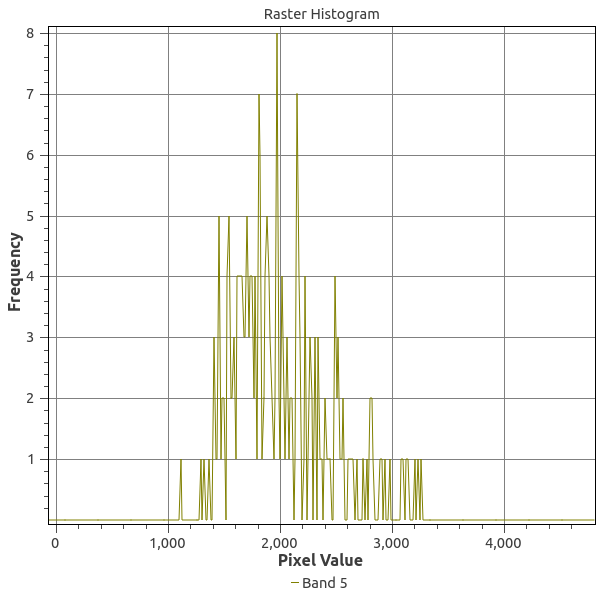
If we examine histograms of segregated water and land areas (below), we can see that there is a sharp divide between the spectral responses of these land cover types in Band 5.

There are two cutoffs we might choose: less than or equal to 500 or 1000 reflectance units. In addition, we might want to sieve the results to reduce commission error. Thus, I experimented with four combinations of thresholds and sieving: a cutoff at either 500 or 1000 reflectance units with or without sieving. We find that sieving had no effect on the performance as measured by precision and recall:
------------------------------------------
Approach      Class     Precision   Recall
-----------   --------- ---------   ------
B5 </= 500    Not water 0.94        1.00
B5 </= 500    Water     1.00        0.96
B5 </= 1000   Not water 0.96        1.00
B5 </= 1000   Water     1.00        0.98
------------------------------------------
And that, on average, a cutoff of 1000 reflectance units performs slightly better:
------------------------------
Approach    Precision   Recall
----------- ---------   ------
B5 </= 500  0.98        0.98
B5 </= 1000 0.99        0.99
------------------------------
Density slicing performs exceptionally well! It performs even better than the naive Bayes estimator. The performance of simple density slicing seems surprising but, then again, we looked at the histogram for Band 5 when choosing the thresholds for slicing and it was very apparent that the land and water pixels were separated at somewhere between 500 and 1000 reflectance units. The real question, then, is whether this relationship holds up across Landsat images (across time and space). In, it works very well for Landsat surface reflectance (SR) data from other dates, though I haven't tried this yet outside of southeast Michigan.
References
- Frazier, P. S., and K. J. Page. 2000. Water Body Detection and Delineation with Landsat TM Data. Photogrammetric Engineering & Remote Sensing 66 (12):1461–1467.