Diagnostics for fixed effects panel models in R

Note: This post has been updated for clarity and to use the Gapminder dataset instead of my old, proprietary example.

I've recently been working with linear fixed-effects panel models for my research. This class of models is a special case of more general multi-level or hierarchical models, which have wide applicability for a number of problems. In hierarchical models, there may be fixed effects, random effects, or both (so-called mixed models); a discussion of the multiple definitions of "fixed effects" is beyond the scope of this post, but Gelman and Hill (2007) or Bolker et al. (2009) are good references for this [4,7]. Fixed effects, in the sense of fixed-effects or panel regression, are basically just categorical indicators for each subject or individual in the model. The way this works without exhausting all of our degrees of freedom is that we have at least two observations over time for each subject (hence: a panel dataset). One further tweak that leads to the "within" estimator discussed in this post is that each subject's panel data are time-demeaned; that is, the long-term average within each subject is subtracted from all measurements for that subject.

Although these models can be fit in R using the the built-in lm() function most users are familiar with, there are good reasons to use one of the two dedicated libraries discussed here:

For large numbers of fixed effects, the function can be intractable and return poor results.
In addition, they clutter in statistical summary() of your model because they're reported alongside any covariates of interest.
The "fixed-effects transformation" (time-demeaning) is applied automatically (and correctly) without you having to transform your data.

In my work, I have about 4000-6000 fixed effects and, fortunately, the R community has delivered two excellent libraries for working with these models: lfe and plm. A more detailed introduction to these packages can be found in [1] and [2], respectively. Here, I'll summarize how to fit these models with each of these packages and how to develop goodness-of-fit tests and tests for the linear model assumptions, which are trickier when working with these packages (as of this writing).

I should state up front that I am going to gloss over much of the statistical red meat, writing, as I usually do, for practitioners rather than statisticians. Also, there are a variety of flavors of models that can be estimated with this framework. I'm going to focus on just one type of model, the panel model by the "within" estimator.

Introduction to Fixed-Effects Panel Models

Fixed-effects panel models have several salient features for investigating drivers of change. They originate from the social sciences, where experimental setups allow for intervention-based prospective studies, and from economics, where intervention is typically impossible but inference is needed on observational data alone. In these prospective studies, a panel of subjects (e.g., patients, children, families) are observed at multiple times (at least twice) over the study period. The chief premise behind fixed effects panel models is that each observational unit or individual (e.g., a patient) is used as its own control, exploiting powerful estimation techniques that remove the effects of any unobserved, time-invariant heterogeneity [3,4]. By estimating the effects of parameters of interest within an individual over time, we can eliminate the effects of all unobserved, time-invariant heterogeneity between the observational units [5]. This feature has led some investigators to propose fixed-effects panel models for weak causal inference [3] as the common problem of omitted variable bias (or "latent variable bias") is removed through differencing. Causal inference with panel models still requires an assumption of strong exogeneity (simply put: no hidden variables and no feedbacks).

The linear fixed-effects panel model extends the well-known linear model, below. The response of individual $i$, denoted $y_i$, is a function of some group mean effect or intercept, $\alpha$, one or more predictors, $\beta x_i$, and an error term, $\varepsilon_i$.

$$ y_i = \alpha + \beta x_i + \varepsilon_i $$

The basic linear fixed-effect panel model can be formulated as follows, where we add an intercept term for each of the individual units of observation, $i$, which are observed at two or more times, $t$:

$$ y_{it} = \alpha_i + \beta x_{it} + \varepsilon_{it} $$

It's important to note that this approach requires multiple observations of each individual. Obviously, if the number of observations $N$ was equal to the number of individuals $i \in M$, we would exhaust the degrees of freedom in our model simply by adding $M$ intercept terms, $\alpha_i + ... + \alpha_M$. With as few as two observations $(t \in [1,2])$ of each subject, however, we've doubled the number of observations and the individual intercept terms now correspond to any time-invariant, idiosyncratic change between those two observations.

This model can be extended further to include both individual fixed effects (as above) and time fixed effects (the "two-ways" model):

$$ y_{it} = \alpha_i + \beta x_{it} + \mu_t + \varepsilon_{it} $$

Here, $\mu_t$ is an intercept term specific to the time period of observation; it represents any change over time that affects all observational units in the same way (e.g., the weather or the news in an outpatient study). These effects can also be thought of as "transitory and idiosyncratic forces acting upon [observational] units (i.e., disturbances)" [3].

Thus, there are two basic kinds of fixed-effects panel models that can be estimated using the "within" estimator. The "unobserved effects" or individual model accounts for unobserved heterogeneity between individuals by partitioning the error term into two parts. One part is specific to the individual unit of observation and doesn't change over time while the other is the idiosyncratic error term, $\varepsilon$, we are familiar with from basic linear models [2]. The second type is an extension of the first, the "two-ways" panel model that includes both individual and time fixed effects.

A further extension of the panel model, one often seen in the literature, is given below.

$$ y_{it} = \alpha_i + \beta x_{it} + \phi z_i + \mu_t + \varepsilon_{it} $$

While $\beta$ and $\epsilon$ do not differ from the meanings in the basic linear model, $\alpha_i$ is the individual fixed effect and $\phi$ is a vector of coefficients for time-invariant, unit-specific effects. These effects can be estimated in a linear model but are removed in some kinds of estimation of panel models ($\phi \equiv 0$). They are removed in estimation through differencing; since each observational unit is used as its own control, we are unable to distinguish between heterogeneity that we didn't observe (and can't account for)—the kind we wish to remove from our model—and known (observed) differences between observational units (e.g., race or sex in patients) [3].

Fitting Fixed-Effects Panel Models in R

Let's look at the Gapminder dataset, a somewhat well-known dataset (owing to the TED talk on the subject) on global development indicators, including life expectancy and per-capita gross domestic product (GDP). You can download the data I used for this example as a CSV file from here. Below is a sample of the Gapminder data.

> head(panel.data)
      country year lifeExp      pop gdpPercap
1 Afghanistan 1952  28.801  8425333  779.4453
2 Afghanistan 1957  30.332  9240934  820.8530
3 Afghanistan 1962  31.997 10267083  853.1007
4 Afghanistan 1967  34.020 11537966  836.1971
5 Afghanistan 1972  36.088 13079460  739.9811
6 Afghanistan 1977  38.438 14880372  786.1134

In this example, the observational units are countries. Here, the country name is the unique identifier for individual subjects (countries) and the year is the identifier for the time period; these are the individual and time fixed effects, respectively. Both the individual and time fixed effects, country and year, must be factors where the levels correspond to the individual and time period identifiers, respectively. I'll investigate to what extent change in life expectancy (lifeExp) is predicted by change in (gdpPercap).

Let's start with lfe. A basic panel model can be with using lfe with the provided felm() method. This approach exploits the vertical-bar in the Wilkinson-Rogers syntax (R formulas) to specify the "levels" by which our panel data are organized. Here, we

library(Matrix)
library(lfe)
m1a <- felm(lifeExp ~ gdpPercap | country, data = panel.data)

We can be more explicit by specifying the contrasts of our model but the result is the same.

m1b <- felm(lifeExp ~ gdpPercap | country, data = panel.data,
  contrasts = c('country', 'year'))

The results are the same. We can see that our predictor, (change in) per-capita GDP is highly significant and we are given two pairs of goodness-of-fit statistics: the multiple and adjusted R-squared for the "full" and "projected" models. The full model is our model with the individual fixed effects included; the projected model is the estimated model where our fixed effects are not included. The full model always performs better than the projected model because the individual fixed effects always explain additional variation in the response: they account for any idiosyncratic differences between each observational unit.

> summary(m1a)

Call:
   felm(formula = lifeExp ~ gdpPercap | country, data = panel.data)

Residuals:
    Min      1Q  Median      3Q     Max
-31.697  -3.424   0.321   3.684  21.106

Coefficients:
           Estimate Std. Error t value Pr(>|t|)    
gdpPercap 4.260e-04  3.114e-05   13.68   <2e-16 ***
---
Signif. codes:  0 ‘***’ 0.001 ‘**’ 0.01 ‘*’ 0.05 ‘.’ 0.1 ‘ ’ 1

Residual standard error: 6.505 on 1561 degrees of freedom
Multiple R-squared(full model): 0.7675   Adjusted R-squared: 0.7464
Multiple R-squared(proj model): 0.1071   Adjusted R-squared: 0.02583
F-statistic(full model): 36.3 on 142 and 1561 DF, p-value: < 2.2e-16
F-statistic(proj model): 187.2 on 1 and 1561 DF, p-value: < 2.2e-16

We can fit the two-ways fixed effects model in lfe simply by adding an additional contrast.

m2 <- felm(lifeExp ~ gdpPercap | country + year, data = panel.data)

Switching to plm, we can fit the two-ways fixed effects model using the plm() function. The plm library doesn't use the vertical bar to specify fixed effects, rather, it requires us to specify the index argument with the variable names of the individual and time fixed effects specified as a tuple (in that order). We also indicate that the model we want to estimate is the within model and that we are estimating twoways effects.

library(Matrix)
library(plm)
m2 <- plm(lifeExp ~ gdpPercap, data = panel.data, model = 'within',
  effect = 'twoways', index = c('country', 'year'))

The output of summary() for plm is different and we get a little more detail in some areas. We see that we have a balanced panel (same number of observations for each individual) over 142 subjects (countries) and 12 time periods (for a total of 1,704 observations).

> summary(m2)

Twoways effects Within Model

Call:
plm(formula = lifeExp ~ gdpPercap, data = panel.data, effect = "twoways",
    model = "within", index = c("country", "year"))

Balanced Panel: n = 142, T = 12, N = 1704

Residuals:
     Min.   1st Qu.    Median   3rd Qu.      Max.
-22.63728  -1.69344  -0.04944   2.00422  10.11005

Coefficients:
             Estimate  Std. Error t-value  Pr(>|t|)    
gdpPercap -7.8017e-05  1.8431e-05 -4.2329 2.442e-05 ***
---
Signif. codes:  0 ‘***’ 0.001 ‘**’ 0.01 ‘*’ 0.05 ‘.’ 0.1 ‘ ’ 1

Total Sum of Squares:    18529
Residual Sum of Squares: 18317
R-Squared:      0.011428
Adj. R-Squared: -0.086154
F-statistic: 17.9177 on 1 and 1550 DF, p-value: 2.442e-05

What we don't see is a goodness-of-fit statistic for the full model. The value of the R-Squared statistic presented here, when compared to the lfe output, is obviously that of the projected model.

Note that the individual effects model can be fit using plm by removing the second variable from the tuple provided to index and specifying an individual effects model:

m2 <- plm(lifeExp ~ gdpPercap, data = panel.data, model = 'within',
  effect = 'individual', index = c('country'))

Goodness-of-Fit for Panel Models

To get a goodness-of-fit metric for the full-model, we have to calculate various sums-of-squares. Returning to our basic statistics, we note that:

$$ R^2 = \frac{SSR}{SST} = \frac{\sum (\hat{y}_i - \bar{y})^2}{\sum (y_i - \bar{y})^2} $$

Where $\hat{y}_i$ and $\bar{y}_i$ are the estimated and mean values, respectively, of $y_i$ and $SSR$ and $SST$ are, respectively, the residual sum-of-squared and total sum-of-squares, related by the following formula:

$$ \sum_{i=1}^n (y_i - \bar{y})^2 = \sum_{i=1}^n (y_i - \hat{y}_i)^2 + \sum_{i=1}^n (\hat{y}_i - \bar{y})^2\\ SST = SSE + SSR $$

Thus, if we can calculate $SSR$ and $SST$, we can calculated R-squared. $SST$ is easily obtained from our model data, as it depends only on the observed values and mean value of our response:

$$ SST = \sum_{i=1}^n (y_i - \bar{y})^2 $$

In R, this is:

sst <- with(panel.data, sum((lifeExp - mean(lifeExp))^2))

Without deriving the fitted values, $\hat{y}$, we can't calculate $SSR$ or $SSE$ directly. I'll get into deriving fitted values later. For now, we can exploit the fact that $SST = SSE + SSR$ so as to derive $SSR$ as the difference between $SST$ and $SSE$, the sum of squared errors. We can then calculate $SSE$ from the least-squares criterion:

$$ SSE = \epsilon '\epsilon = (y - X\beta )' (y - X\beta ) $$

In R, this is:

m1.sse <- t(residuals(m1)) %*% residuals(m1)

Putting this altogether, in R, we can derive R-squared as follows. Recall that, here, lifeExp signifies my dependent or response variable.

> sst <- with(panel.data, sum((lifeExp - mean(lifeExp))^2))
> m1.sse <- t(residuals(m1)) %*% residuals(m1)
> (sst - m1.sse) / sst

          [,1]
[1,] 0.7675404

We obtain $R^2 = 0.9355361$, which, compared to the R-squared estimated for the full (individual fixed effects) model by lfe, is a pretty good estimate. Why bother calculating this when lfe does it for free? In my work, I found that lfe and felm() choked on some two-ways panel models I was fitting but, if that's not a problem for you, just use lfe. In addition, lfe doesn't provide adjusted R-squared, which is a better estimate between models with differing numbers of parameters.

Adjusted R-squared is defined as:

$$ \bar{R}^2 = 1 - (1 - R^2)\frac{n-1}{n-p-1} = 1 - \frac{SSR(n-1)^{-1}}{SST(n-p-1)^{-1}} $$

Provided we have $R^2$, here denoted m1.r2, we can calculate $n$, the number of observations, and the adjusted R-squared statistic in R as follows:

m1.r2 <- (sst - m1.sse) / sst
N <- dim(panel.data)[1]
1 - (1 - m1.r2)*((N - 1)/(N - length(coef(m1)) - 1))

Calculating Fitted Values

You might think of extracting the fitted values with the fitted() function in R. It's not clear to me that this works; the values I get from fitted() for any of the models I've worked with are too small. Unfortunately, there's no documentation I can find as to how the fitted() function performs on plm() model instances; i.e., ?fitted.plm returns nothing, nor does a quick search online.

Luckily, we can recall from elementary statistics that the fitted values can also be calculated as the difference between our observed values and the residuals.

panel.data$lifeExp - residuals(m1)

A quick fitted-versus-observed plot shows we're not doing too badly with this model.

# An example fitted-vs-observed plot
plot(panel.data$lifeExp - residuals(m1), panel.data$lifeExp, asp = 1)
abline(0, 1, col = 'red', lty = 'dashed', lwd = 2)

Calculating Fitted Values for Hypothesis Testing

What if you want to conduct hypothesis testing using proposed values for one or more main effects? For instance, within the Gapminder example, we might ask the question: what is a certain country's per-capita GDP grew at a different rate than it actually did? This is harder to do because the predict() function in R doesn't work out-of-the-box with felm() or plm() models.

This is a clearly made-up example, but let's say that per-capita GDP world-wide was 10% lower in 2002 and 2007 than we actually observed. Below, I use the dplyr library to transform the data this way. If you're unfamiliar with dplyr, just know that, below, I am scaling back per-capita GDP estimates in 2002 and 2007 by 10%, merging those years with the rest of the data, and then formatting my data frame so it is arranged the same way as the original.

library(dplyr)
panel.data2 <- panel.data %>%
  filter(year >= 2002) %>%
  mutate(gdpPercap = gdpPercap - (gdpPercap * 0.10)) %>%
  rbind(filter(panel.data, year < 2002)) %>%
  arrange(country, year)

Now, let's test this hypothesis with plm(). Let's also develop a slightly more complex fixed effects regression model. We have data on population in each year, and this might have something to do with life expectancy; it's a time-varying estimate of our system, so let's include it in the model.

> m3 <- plm(lifeExp ~ gdpPercap + pop, data = panel.data, model = 'within',
  effect = 'individual', index = c('country'))
> coef(m3)
   gdpPercap          pop
3.936623e-04 6.196916e-08

We get a similar, though slightly smaller estimate of the effect of (change in) per-capita GDP on (change in) life expectancy. Now, how can we obtain the fitted values using the existing model, but new data? Again, linear algebra helps us find the answer. Recall the formula for the individual fixed effects model we saw earlier.

$$ y_{it} = \alpha_i + \beta x_{it} + \phi z_i + \varepsilon_{it} $$

Because $z_i$ is really just a repeated index for each subject (observed multiple times), every term is additive other than the main effects $\beta x_{it}$. This means it is easy to calculate the fitted values for a new set of values (for the same subjects). In the case of the individual fixed effects model, we compute the product of the main effects and the new observations of our $X$ matrix and add it to the fixed effects, which need to be repeated in the order they appear in the original design matrix. Because our Gapminder data are ordered by country name, then year, for 12 years, we need to repeat each country fixed effect 12 times. Below, the function fixef() allows us to extract the country fixed effects from a given model.

# Get the new X matrix with our new (hypothetical) values
new.X <- as.matrix(select(panel.data2, gdpPercap, pop))

# Repeat each fixed effect 12 times (12 observations for each subject)
fe <- rep(as.numeric(fixef(m3)), each = 12)

# Compute our predictions
preds <- (new.X %*% coef(m3)) + fe

It's important to note that this is not "out-of-sample prediction." That wouldn't make sense for a fixed effects regression and would, in fact, be misleading. We have fit fixed effects for each of our subjects (here, countries) and it wouldn't make sense to use this model for a different set of subjects. What we're doing here is testing a counterfactual, e.g., suppose that $X$ has a different value, what would be the effect on $Y$?

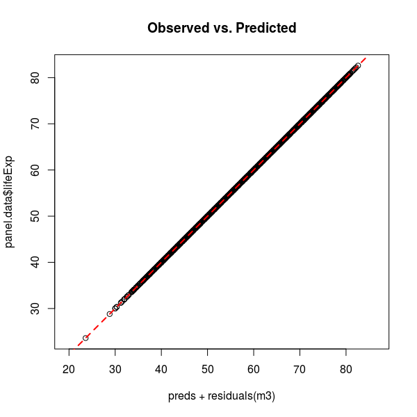
We can confirm we've calculated the fitted values correctly by returning to the original dataset and adding the residuals to our fitted values. The residuals add the random variation of our original, observed response back into our model; the result is a perfect fit, as seen in how the plot points line up perfectly along the 1:1 line.

old.X <- as.matrix(select(panel.data, gdpPercap, pop))

# Repeat each fixed effect 12 times (12 observations for each subject)
fe <- rep(as.numeric(fixef(m3)), each = 12)

# Compute our predictions THIS TIME with the residuals
preds <- (new.X %*% coef(m3)) + fe + residuals(m3)

plot(preds, panel.data$lifeExp, asp = 1)
abline(0, 1, col = 'red', lty = 'dashed', lwd = 2)

I haven't been able to figure out how to do this for the two-ways model (with time fixed effects) yet. The result should require the addition of the time fixed effects, but I'm not getting the right result.

The above examples work for lfe::felm() models, too, as fixef() can also extract the fixed effects models from the lfe package.

Model Diagnostics

Two critical assumptions of any linear model, including linear fixed-effects panel models, are constant variance (homoskedasticity) and normally distributed errors [6]. We might also want to determine the leverage of our observations to see if there are any highly influential points (which might be outliers). In addition, since we're working with spatial data (in this case), we'll do a crude check for spatial autocorrelation in the residuals, which, if present, would be problematic for inference.

Normally Distributed Errors

This is a quick check using a couple of built-in functions. We want to determine that the curve of our residuals in a QQ-Normal plot follow a straight line. Some curvature in the tails is to be expected; it is a somewhat subjective test but this assumption is also commonly satisfied with observational data.

qqnorm(residuals(m3), ylab = 'Residuals')
qqline(residuals(m3))

We might also examine a histogram of the residuals.

hist(residuals(m1), xlab = 'Residuals')

Constant Variance

Here, a plot of the residuals against the fitted values should reveal whether or not there is non-constant variance (heteroskedasticity) in the residuals, which would violate one of the assumptions of our linear model. We look for whether or not the spread of points is uniform in the y-direction as we move along the x-axis (constant variance along the x-axis).

plot(preds, residuals(m3))

Checking for Influential Observations

To derive the leverage of the observations, we wish to derive hat matrix (or "projection matrix") from our linear model. This is the matrix given by the linear transformation by which we obtained the estimated coefficients for our model, $\beta$.

$$ X\hat{\beta} = X(X^T X)^{-1} X^Ty = Py $$

Where $X$ is the design matrix (matrix of explanatory variables) and $y$ is the vector of our observed response values. The hat (or projection) matrix is denoted by $P$. The diagonal of this $N\times N$ matrix (diag(P) in R) contains the leverages for each observation point.

In R, we use matrix multiplication and the solve() function (to obtain the inverse of a matrix). With the faraway package, we can draw a half-normal plot which sorts the observations by their leverage.

X <- panel.data[,c('lifeExp', 'gdpPercap')]
X <- as.matrix(X)
P = X %*% solve(t(X) %*% X) %*% t(X)

require(faraway)
# Create `labs` (labels) for 1 through 1704 observations
halfnorm(diag(P), labs = 1:1704, ylab = 'Leverages', nlab = 1)

This theory and approach are based on the general linear model and ordinary least squares (OLS) regression, corresponding to models built with lm() in R. Some adjustment may be necessary to calculate leverage correctly for fixed effects models. However, this approach based on OLS seems to work pretty well; the points with the most leverage I find correspond to Kuwait in the 1950s through 1970s, a period when the country's per-capita GDP went on a roller coaster, reaching the highest value seen in the dataset.

If we need to remove influential observations, in order to maintain a balanced panel, it's important to remove all of the observations for that individual; that is, to remove that individual entirely from the panel, rather than just the observation(s) at those time period(s). In R, we do this by querying those points that have an influence above a certain threshold, say 0.004; here, the individual units of observation are denoted by unique country names.

panel.data.mod <- subset(panel.data,
  !(country %in% panel.data[names(diag(P)[diag(P) > 0.004]), 'country']))

References

Gaure, S. 2013. lfe: Linear Group Fixed Effects. The R Journal 5(2):104–117.
Croissant, Y., and G. Millo. 2008. Panel data econometrics in R: The plm package. Journal of Statistical Software 27(2):1–43.
Halaby, C. N. 2004. Panel Models in Sociological Research: Theory into Practice. Annual Review of Sociology 30(1):507–544.
Gelman, A., and J. Hill. 2007. Data Analysis Using Regression and Multilevel/Hierarchical Models. New York, New York, USA: Cambridge University Press.
Allison, P. D. 2009. Fixed Effects Regression Models ed. T. F. Liao. Thousand Oaks, California, U.S.A.: SAGE.
Crawley, M. J. 2015. Statistics: An Introduction Using R 2nd ed. Chichest, West Sussex, United Kingdom: John Wiley & Sons.
Bolker, B. M., M. E. Brooks, C. J. Clark, S. W. Geange, J. R. Poulsen, M. H. H. Stevens, and J. S. S. White. 2009. Generalized linear mixed models: a practical guide for ecology and evolution. Trends in Ecology and Evolution 24(3):127–135.