Recently, I was working with a colleague on a project involving time series observations of neighborhoods in Los Angeles. We wanted to see if there were patterns in the time series data that described how similar neighborhoods evolved in time. For multivariate data, this is a great application for unsupervised learning: we wish to discover subgroups among either among the variables (obtaining a more parsimonious description of the data) or among the observations (grouping similar samples together) [1]. My colleague described what we needed as a "PCA for time series."
Though I was familiar with principal components analysis (PCA), I didn't know what to expect from applying PCA to a time series.
- How should the data be structured?
- How does the approach compare to digital signal processing techniques like singular spectrum analysis (SSA)?
- How can PCA and SSA be implemented in the R environment?
Here, I attempt to provide a brief introduction to PCA, SSA, and their implementations in R, along with the relevant considerations of their similarities and differences. It may seem that SSA is coming out of left field; what the hell is it? This investigation was prompted by a question about PCA, after all. However, SSA and PCA have interesting similarities and differences that I think merit their joint discussion, at least at the level I'm capable of here.
Principal Components Analysis
The objective of PCA is to "provide the best \(m\)-dimensional approximation (in terms of Euclidean distance)" [1] to each observation in a \(p\)-dimensional dataset, where \(p > m\). This characterization places PCA in a list of other "dimesionality reduction" techniques that seek to describe a set of data using fewer variables (or dimensions/ degrees of freedom) than were measured. A lower-dimensional description of a dataset has obvious benefits for data compression---fewer variables used to describe the data means fewer columns in a table or fewer tables in a data cube---but it can also reveal hidden structure in the data.
What we obtain from PCA is a coordinate transformation; our data are projected from their original coordinate system (spanned by the variables we measured) onto a new, orthogonal basis. In this way, correlation that may have existed between the columns in our original data is eliminated. The new variables, referred to as principal components, in this new coordinate system can be hard to interpret and may not have a physical meaning. They are intrinsicaly ordered by the amount of variance in the data they explain.
PCA can be implemented in one of two ways:
- Through a spectral decomposition of the covariance ("unstandarized" PCA) or correlation matrix ("standardized" PCA) [1];
- Through a singular value decomposition (SVD) of the data matrix, \(X\).
PCA is sometimes referred to as being "standardized" or "unstandardized" [2]. In standardized PCA, the correlation matrix is used in place of the covariance matrix of unstandardized PCA. If the variables in \(X\) are measured on different scales, their corresponding variances will also be scaled differently, which can put unequal weight on one or more of our original variables. This weight is often unjustified. James et al. (2013), for example, describe a dataset where one of the variables in an urban crime dataset, the rate of criminal assaults, has a much larger variance than the other variables, including the rates of rape and murder, simply because they occur far more often than other crimes. Figure 10.3 in their book is an excellent visual aid here. In general, we want to both mean-center and standardize the variables in our data matrix, \(X\), prior to PCA. If we're using the SVD approach, mean-centering and standardizing our data matrix, \(X\), is equivalent to using the correlation matrix, rather than the covariance matrix, in spectral decomposition.
It's important for both the description of PCA and, later, of SSA, to provide some background on matrix decomposition.
Spectral or Eigenvalue Decomposition
Spectral decomposition, also referred to as eigenvalue decomposition, factors any diagonalizable (square) matrix into a canonical form. The oft-described "canonical form" makes intuitive sense, here, in a larger discussion of PCA because a canonical form is precisely what we wish to find in our original, messy dataset.
Given a multivariate dataset \(X\) as an \(n\times p\) matrix, where the columns \(X_i,\, i\in \{1,\cdots ,p\}\) represent distinct variables and the rows represent different observations or samples of each of the variables, the spectral decomposition of the covariance matrix can be written as:
Where \(A\) is a real, symmetric matrix and the columns of \(Q\) are the orthonormal eigenvectors of \(A\) [3]. \(\Lambda\) is a diagonal matrix and the non-zero values correspond to the eigenvalues. Elsner and Tsonis (1996) provide a concise introduction to the intuition behind eigenvectors and eigenvalues.
Singular Value Decomposition
Singular value decomposition is a generalization of spectral decomposition. Any \(m\times n\) matrix \(X\) can be factored into a composition of orthogonal matrices, \(U\) and \(V^T\), and a diagonalizable matrix \(\Sigma\):
The columns of the \(m\times m\) matrix \(U\) are the eigenvectors of \(XX^T\) while the columns of the \(n\times n\) matrix \(V\) are the eigenvectors of \(X^TX\). The columns of \(U\) and \(V\) are also called the "left" and "right" singular vectors. The singular values on the diagonal of \(\Sigma\) are the square-roots of the non-zero eigenvalues of both the \(XX^T\) and \(X^TX\) matrices [5].
In PCA, the "right singular vectors," the columns of the \(V\) matrix, of an SVD are equivalent to the eigenvectors of the covariance matrix [4]. Also, the eigenvalues of the covariance matrix correspond to the variance explained by each respective principal component.
PCA can be implemented in R in a few different ways for a data matrix X.
# SVD of the (scaled) data matrix; the name `v` is the matrix of PCs as column vectors
svd(scale(X))$v

# Spectral decomp. of the covariance/ correlation matrix;
# `vectors` has matrix of PCs as column vectors
eigen(cor(X))$vectors

# Built-in tool for PCA; `rotation` has matrix of PCs as column vectors
prcomp(X, scale. = T)$rotation
Singular Spectrum Analysis
Singular spectrum analysis (SSA) is a technique used to discover oscillation series of any length within a longer (univariate) time series. Oscillations are of interest, generally, because they are associated with various signals of interest: in ecology, it could be seasonal/ phenological change; in physics or engineering, it could be a mechanical or electrical wave.
"An oscillatory series is a periodic or quasi-periodic series which can be either pure or amplitude-modulated. Noise is any aperiodic series. The trend of the series is, roughly speaking, a slowly varying additive component of the series with all the oscillations removed." - Golyandina et al. (2001)
Unlike PCA, SSA is generally performed on a univariate dataset: a single variable observed at multiple points in time. There is a multivariate form of SSA, sometimes called M-SSA, but it is beyond my current understanding. Univariate SSA is a lot like PCA for univariate time series data.
There are a couple of different approaches to setting up SSA. One way, described in Elsner and Tsonis' (1996) excellent and very accessible book, begins by constructing the trajectory matrix. The trajectory matrix is the \(n\times m\) matrix whose row vectors are every consecutive \(m\)-tuple, or every window of length \(m\), in the time series.
"By using lagged copies of a single time series, we can define the coordinates of the phase space that will approximate the dynamics of the system from which the time record was sampled. The number of lags is called the embedding dimension." - Elsner and Tsonis (1996)
A general formula for the number of rows in the trajectory matrix is \(n = n_t-m+1\), where \(n_t\) is the length of the original time series vector. For instance, a time series of 6 observations with an embedding dimension of \(m=3\) will have \(n=4\) possible combinations of 3 consecutive values from among 6 ordered values. This means there are 4 rows in the trajectory matrix. The trajectory matrix is definitely not linearly independent.
"[The trajectory matrix] contains the complete record of patterns that have occurred within a window of size [m]." - Elsner and Tsonis (1996)
The trajectory matrix is the matrix whose \((i,j)\) element is defined:
Where \(x\) is some ordered, time series vector.
It is customary to normalize the elements of the trajectory matrix by \(n\), the number of windows. That is, for a single time series record \(v = \{v_1, v_2, \cdots, v_n\}\), the trajectory matrix for an embedding dimension \(m\) could be written as:
The lagged-covariance matrix is then defined:
There are two ways to perform SSA as a matrix decomposition:
- Through the spectral decomposition of the (normalized) lagged-covariance matrix, \(S = X^TX\). Here, \(X\) is not the data matrix, but the trajectory matrix; the matrix formed by all possible time windows of length \(m\). The normalization factor used is \(1/\sqrt{n}\), where \(n = n_t-m+1\) is the number of time windows of length \(m\) taken from a time series vector of length \(n_t\).
- Through the singular value decomposition (SVD) of the trajectory matrix [4], \(X\), taking the right singular vectors, or \(V\) in the SVD given by \(S + UG(V^T)\).
It's easy to see why these two methods are equivalent, if we recall that the right singular vectors of an SVD on \(X\) correspond to the eigenvectors of the matrix \(X^TX\). The spectral decomposition approach is described in detail by Elsner and Tsonis (1996) while the SVD approach is described by Golyandina et al. (2001).
SSA, Stationarity, and Autocorrelation
If the underlying signal is contaminated only by white noise (AR0 noise), then the dominant eigenvalutes will be associated with oscillations in the time series record. If the noise is autocorrelated (red or AR1 noise), however, "then dominant eigenvalues in the singular spectrum will characterize both the noise and signal components of the record" [3]. It should also be noted that higher-order autocorrelation structures, AR2 and AR3, do produce oscillations.
SSA versus PCA
You should immediately notice one similarity between PCA and SSA. They both can be computed through either a spectral decomposition of a covariance matrix or through an SVD of the data matrix, taking careful note that the data matrix in SSA is the trajectory matrix for a single time series record.
Elsner and Tsonis (1996) claim that aside from the difference between the composition of \(X\), i.e., between the trajectory matrix (containing lagged windows of a univariate time series) in SSA and the data matrix of PCA (containing multivariate time series records), "there is no difference between the expansion [of the data set] used in classical PCA and the expansion [of the data set] in SSA." More specifically, PCA can be defined as the spectral decomposition of the covariance matrix \(X^TX\) whereas SSA can be defined as the spectral decomposition of the (normalized) lagged-covariance matrix, which is also designated \(X^TX\); however, in PCA, \(X\) is the data matrix while in SSA \(X\) is the trajectory matrix.
The difference between the structure of the matrix \(X\) in PCA versus SSA is precisely what contributes to their different behaviors.
In PCA, the matrix consists of a single variable observed at multiple locations (a multivariate time series dataset, where the variables are different spatial locations) and the resuling components are termed spatial principal components [3]. In SSA, the matrix consists of a single time series (a single variable observed in a single location) "observed" at different time windows; the resulting components derived through SSA could be termed temporal principal components.
In the digital signal processing community, PCA (as a spectral decomposition of the correlation, not covariance, matrix) is also known as Karhunen–Loève (K-L) expansion.
Implementation in R
I'll demonstrate PCA and SSA in R using two different time series datasets, as they do have two, central assumptions about time series data that differ:
- In PCA, we necessarily have one variable observed over time at multiple locations or among multiple sample units;
- In (univariate) SSA, we necessarily have one variable observed over time as a single record, or in a single location.
For SSA, I'll use the LakeHuron dataset, bundled with R and described here; it consists of observations of the water level in Lake Huron (one place) over time.
For PCA, I couldn't find a built-in dataset that was adequate, so I'm using a series of home sale price observations in multiple neighborhoods in Los Angeles from 1989 to 2010.
PCA for Time Series Data in R
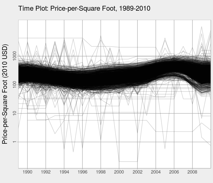
The first thing we want to do with time series data in R is create a time plot to look at the (mean) behavior over time. Here, a time plot of the price-per-square foot data indicates there is an overall regional oscillation in prices. In Los Angeles, it appears that prices peak just before the subprime mortgage crisis of 2006-2007.
The set up our data for PCA, we need to make sure the data frame is in "wide format," i.e., the years span the columns.
More formally, the elements of the \(X\) matrix are generated from sampling a time series \(T\) at location \(i\) and at time \(j\):
Deriving the Spatial Principal Components
The PCA here is performed using a singular value decomposition of the mean-centered and scaled data matrix, \(X\). We then create a screeplot, which shows the proportion of variance explained by each principal component.
pca.price.only <- svd(scale(my.data)))

plot((pca.price.only$d^2 / sum(pca.price.only$d^2))[1:10], type = 'b',
  log = 'y', main = 'Screeplot (Log10): PCA on Price Data Only',
  ylab = 'Proportion of Variance Explained', xlab = 'No. of Principal Components')
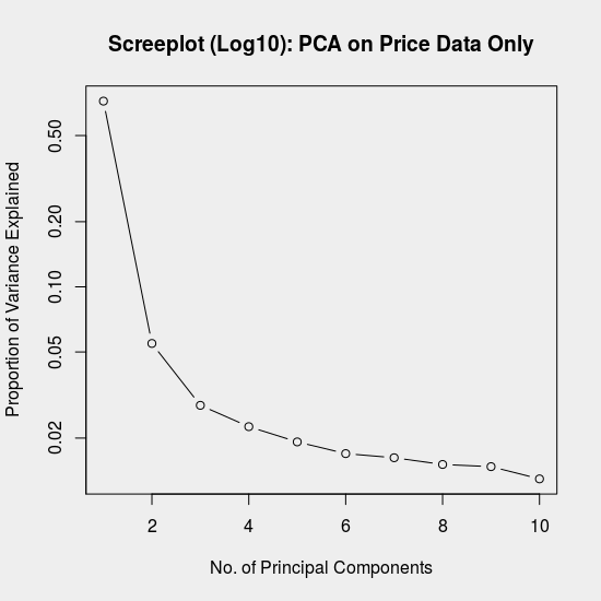
Recall that the variance explained is proportional to the corresponding eigenvalue, among \(P\) total eigenvalues. The proportion of total variance, \(d_i\), attributable to principal component \(i\), can thus be calculated from the SVD, \(X = U\Sigma V^T\), as:
The screeplot is helpful for identifying how many distinct components to the variance exist. If our aim with PCA is dimensionality reduction or compression, we can use this plot to decide how many principal components are needed to approximate the original data.
Visualizing the Spatial Principal Components
We'll examine the first four (4) principal components. By plotting the right singular vectors, we can visualize the loadings of each variable on each of the principal components. Recall that because the "variables" in this time-series dataset are different years of observation, what the loadings here represent is the contribution of each year to the spatial pattern of variance. That is why Elsner and Tsonis (1996) refer to these as spatial principal components.
pca.price.components <- data.frame(
  year = seq.int(1989, 2010),
  Price.PC1 = pca.price.only$v[1:22,1],
  Price.PC2 = pca.price.only$v[1:22,2],
  Price.PC3 = pca.price.only$v[1:22,3],
  Price.PC4 = pca.price.only$v[1:22,4])

require(stringr)
pca.price.components %>%
  gather(key = 'PCs', value = 'loading', -year) %>%
  mutate(
    variable = substr(PCs, 1, 5),
    PCs = str_replace(PCs, '(Price|Loans)\\.', '')) %>%
  ggplot(mapping = aes(x = year, y = loading)) +
  geom_line(size = 1) +
  facet_wrap(~ PCs) +
  labs(title = 'Loadings on Principal Components: Log10 Price-per-Square Foot',
    x = '') +
  theme_linedraw()
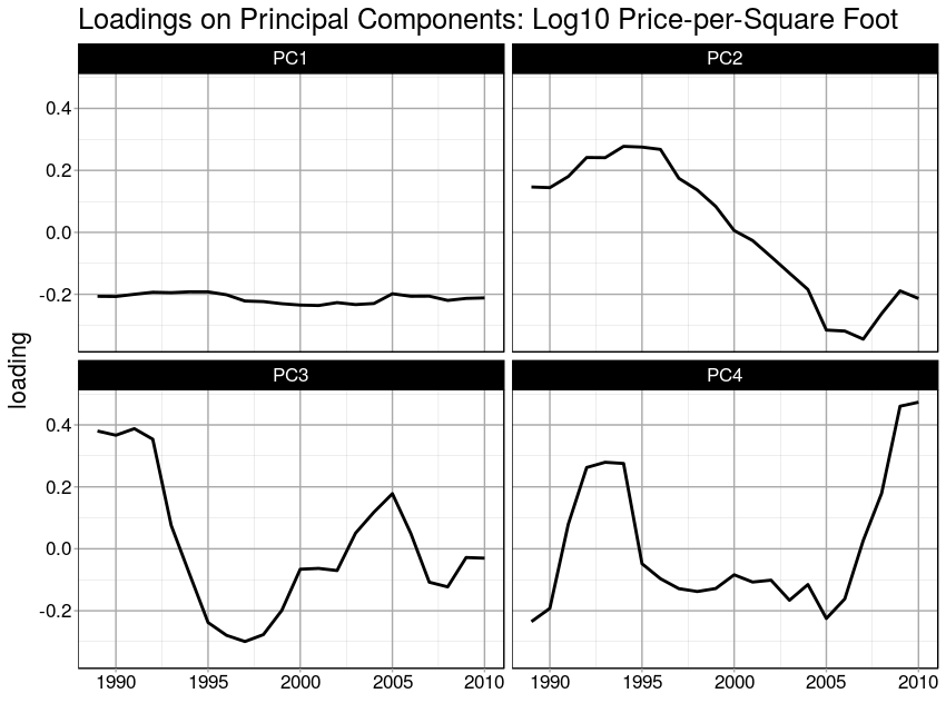
Eastman and Fulk (1993) conducted a standardized PCA on vegetation in Africa and provide an excellent interpretation of the loadings on the spatial principal components:
"If a [year] shows a strong positive correlation with a specific component, it indicates that that [year] contains a latent (i.e., to some extent hidden or unappearnt) spatial pattern that has strong similarity to the one depicted in teh component image. Similarly, a strong negative corerlation indicates that the monthly image has a latent pattern that is the inverse of that shown (i.e., with positive and negative anomalies reversed." [2]
When the first principal component is essentially constant over time, as it is in the case of PC1 in this example, it indicates that the dominant variation in the data occurs over space. In this example, it means that there is more variation in sale prices between L.A. neighborhoods in any year than over time for all neighborhoods.
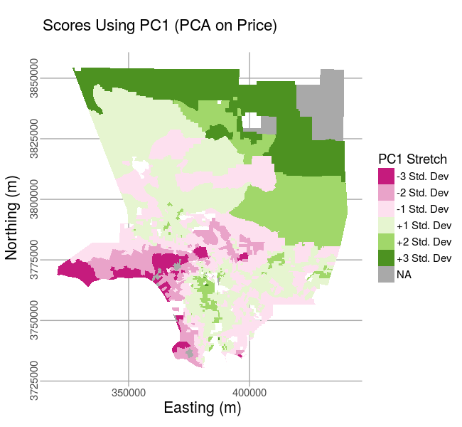
Mapping the spatial principal component scores, or the original values projected onto the principal components, might aid intepretation. The scores can be obtained for a one or more principal components, up to \(m\) total principal components, as the product of a subset of the columns, \(W\), and the mean-centered and scaled time-series data, \(Z\):
# Mean-center and scale the original data values
var.price.scaled <- as.matrix(scale(select(var.by.year.clean, starts_with('price'))))

# Calculate the rotated values
pca.price.spatial <- matrix(nrow = nrow(var.price.scaled),
  ncol = ncol(pca.price.only$v))
for (i in 1:ncol(pca.price.spatial)) {
  pca.price.spatial[,i] <- var.price.scaled %*% as.matrix(pca.price.only$v[,i])
}
When we map the scores, here presented as the number of standard deviations around the mean score, for the first principal component, we see the dominant, time-invariant (or aggregate) spatial variation in price. If we make a similar map for PC2, we can compare it to the loadings plot above. The areas with positive correlations in the map follow the time trend indicated in the loadings for PC2; the areas with negative corerlations in the map follow the inverse of that PC2 time trend.
SSA for Time Series Data in R
For SSA, which assumes weak stationarity, we want to look at the first differences of the LakeHuron data.
Differencing is easy in R with the diff() function.
data(LakeHuron)
plot(LakeHuron, main = 'Lake Huron Water Levels', xlab = 'Lake Level (ft)')
plot(diff(LakeHuron), main = 'Lake Huron Water Levels: First Difference',
  xlab = 'Lake Level (ft)')
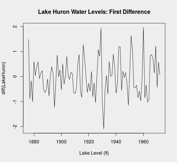
We might take a moment to confirm that first-differencing of the water levels data is adequate to produce a time series that is first-order stationary.
The acf() function in R is a good tool for visual inspection of time series data.
The resulting plot shows very low correlation after the zeroth lag (lag \(= 0\)), which is encouraging.
acf(diff(LakeHuron), type = 'covariance')
Construction of the Trajectory Matrix
We'll construct two different trajectory matrices, investigating 10- and 25-year windows. Recall that the trajectory matrix is an \((n-m+1)\times m\) matrix for an embedding dimension of \(m\).
# Construct the trajectory matrix (Elsner and Tsonis 1996, p.44)
traj10 <- matrix(nrow = length(diff(LakeHuron)) - 10 + 1, ncol = 10)
traj25 <- matrix(nrow = length(diff(LakeHuron)) - 25 + 1, ncol = 25)
To populate the matrices, we can use a for loop to calculate all the windows of length \(m\) in the dataset.
Recall that the \((i,j)\) element of the trajectory matrix is given by \(x_{i+j-1}\), where \(x\) is our first-differenced LakeHuron time series.
for (i in 1:nrow(traj10)) {
  for (j in 1:ncol(traj10)) {
    traj10[i, j] <- diff(LakeHuron)[i + j - 1]
  }
}
The Lagged-Covariance Matrix
We next construct the lagged-covariance matrix by performing a spectral decomposition of the lagged covariance matrix. Recall that this is formed from the trajectory matrix \(X\) as \(X^TX\). Note that we normalize each matrix by one over the square-root of the number of time windows (the number of rows in the trajectory matrix).
S.traj10 <- (t(traj10) * 1/sqrt(nrow(traj10))) %*% (traj10 * 1/sqrt(nrow(traj10)))
S.traj25 <- (t(traj25) * 1/sqrt(nrow(traj25))) %*% (traj25 * 1/sqrt(nrow(traj25)))
Derivation of the Eigenvectors
Recall that we can get the eigenvectors in one of two ways. The first way, perhaps more straightforward, is through a spectral (eigenvalue) decomposition of the lagged-covariance matrix.
# Spectral decomposition of the lagged covariance matrix (columns are eigenvectors)
S.traj10.eigen <- eigen(S.traj10, symmetric = T)$vectors
Alternatively, we could take an SVD of the trajectory matrix, keeping the right singular vectors.
# SVD of the trajectory matrix
S.traj10.by.svd <- svd(traj10)
We can confirm these are equivalent up to a sign change as follows.
all.equal(sapply(S.traj10.by.svd$v, abs), sapply(S.traj10.eigen, abs))
The two approaches may show sign differences in the resulting eigenvectors because the definition of the direction of the coordinate system is arbitrary. The same is true in PCA [1].
"Each principal component loading vector is unique, up to a sign flip...The signs may differ because each principal component loading vector specifies a direction in p-dimensional space: flipping the sign has no effect as the direction does not change." - James et al. (2013)
Visualizing the Temporal Principal Components
The temporal principal components [3], which correspond to the eigenvectors of the lagged-covariance matrix, are more easily visualized if we wrap up our results in an R data frame.
S.traj10.eigen <- eigen(S.traj10, symmetric = T)$vectors
dat.traj10 <- as.data.frame(S.traj10.eigen)
colnames(dat.traj10) <- 1:ncol(dat.traj10)
dat.traj10$time <- 1:ncol(dat.traj10)

require(dplyr)
require(tidyr)
require(ggplot2)
dat.traj10 %>%
  gather(key = 'eigenvector', value = 'value', -time) %>%
  mutate(eigenvector = ordered(eigenvector, levels = 1:1000)) %>%
  ggplot(mapping = aes(x = time, y = value)) +
  geom_line(size = 0.8) +
  facet_wrap(~ eigenvector) +
  theme_linedraw()
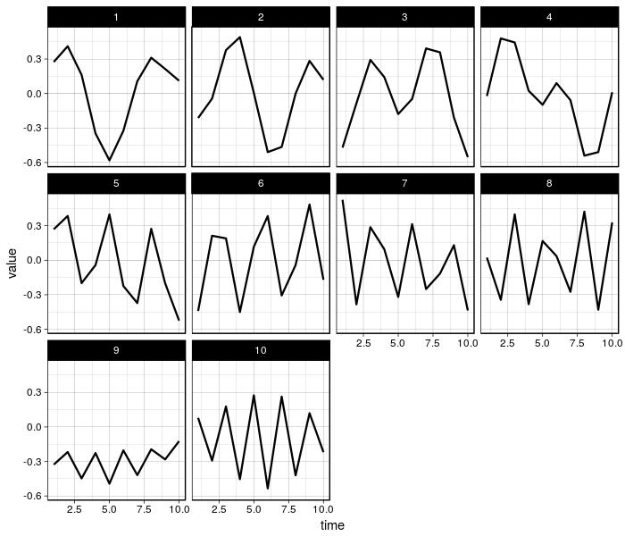
Like PCA, interpretation of SSA results can be subjective. SSA results may be even harder to interpet because every temporal principal component is some oscillation. A more straightforward goal with SSA is smoothing, achieved in the reconstruction of the original signal using a subset of the components.
Conclusion
This is my take on SSA, PCA, and how they compare for different applications.
PCA is a well-established tool for exploratory visualization and analysis of multivariate data. It's particularly valuable for high-dimensional data (lots of columns). For time series data, it may be less useful if there is more variation between spatial units/ sample units than over time.
SSA is a neat technique for discovering oscillations in time series data but it is tricky to get right. Oscillations may correspond either to signal or to noise and you need to know more about the data generating mechanism in order to distinguish the two. The assumption of first-order stationarity might also pose a problem for certain time series datasets. As a result, SSA may be better for smoothing and forecasting time series data than discovering canonical trajectories. It's also clear that SSA requires longer time series than PCA for practical use.
References
- James, G., D. Witten, R. Tibshirani, and T. Hastie. 2013. An Introduction to Statistical Learning with Applications in R. New York, New York, USA: Springer Texts in Statistics.
- Eastman, R., and M. Fulk. 1993. Long sequence time series evaluation using standardized principal components. Photogrammatic Engineering & Remote Sensing 59(6):991–996.
- Elsner, J., and A. Tsonis. 1996. Singular spectrum analysis: a new tool in time series analysis. New York and London: Plenum Press.
- Golyandina, N., V. Nekrutkin, and A. Zhigljavsky. 2001. Analysis of Time Series Structure: SSA and Related Techniques. Washington, D.C., U.S.A.: Chapman and Hall/CRC.
- Strang, G. 1988. Linear Algebra and its Applications. Orlando, Florida. Harcourt Brace Jovanovich, Inc. 3rd ed.