I've been using Google Earth Engine recently to scale up my remote sensing analyses, particularly by leveraging the full Landsat archive available on Google's servers. I've followed Earth Engine's development for years, and published results from the platform, but, before now, never had a compelling reason to use it. Now, without hubris, I can say that some of the methods I'm using (radiometric rectification of thousands of images in multi-decadal time series) are already straining the limits of the freely available computing resources on Google's platform. After an intensive pipeline that merely normalizes the time series data I want to work with, I don't seem to have the resources to perform, say, a pixel-level time series regression on my image stack. Whatever the underlying issue (is it never quite clear with Earth Engine), regressions as the scale of 30 meters (a Landsat pixel) for the study area I'm working on, following the necessary pre-processing, hasn't been working.
I started wondering if I could calculate the regressions myself in (client-side) Python. Image exports from Earth Engine used to be infeasible but they have vastly improved and, recently, I've been able to schedule export "tasks," monitor them using a command-line interface, and download the results directly from Google Drive. With the pre-processed rasters downloaded to my computer, I turned to NumPy to develop a vectorized regression over each pixel in a time series image stack. Here, I describe the general procedure I used and how it can be scaled up using Python's concurrency support, pointing out some potential pitfalls associated with using multiple processes in Python.
A Note on Concurrency
I recently attended part of a workshop run by XSEDE, a collaborative organization funded by the National Science Foundation to further high performance computing (HPC) projects. The introductory material was very interesting to me, not because I was unfamiliar with HPC, but because of the many compelling reasons for learning and using concurrency in scientific computing applications.
First and perhaps best known among these reasons, is that Moore's Law, which predicts a doubling in the number of transistors on a commercially available chip every two years, started to level off at around 2004. The rate is slowing, and in the graph at the top of Wikipedia's page on the Law, you can already see the right-hand turn this trajectory is making. This is largely due to real physical limitations that chip developers are starting to encounter. The gains in the number of transistors per chip have come from making transistors progressively smaller; the smaller the transistor, the more heat (density) that must be dissipated.
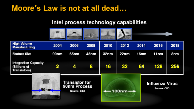
According to one of XSEDE's instructors during the recent "Summer Bootcamp" that I attended, computer chips today are tasked with dissipating heat, in terms of watts-per-square meter, on the order of a nuclear reactor! Keeping things from melting has become the main concern of chip design. But, as we reduce the clock rate and the voltage required to run the chip, we can reduce the amount of heat generated. There is a reduction in performance, but if we add a second chip and run both at a lower voltage, we can get more performance for the same total amount of voltage used by the single chip. Lower voltage means less power consumed and less heat generated [1].
In short, because of physical limitations to chip design and the demand for both power and heat dissipation, commercially available computers today almost exclusively ship with two or more central processing units (CPUs or "cores") running at a clock speed (measured in GHz) than many chips sold just a few years ago. When I was building computers as a kid in the early 2000s, I could buy Intel chips with clock speeds in excess of 3 GHz. A quick search on any vendor's website (say, Dell Corporation's) today, however, reveals that clock speeds haven't really budged: their new desktops ship with cores clocked at 3-4 GHz. The new computers are still "faster" for many applications, however, for the reasons I just discussed: multiple cores running simultaneously.
Multiple Threads, Multiple Processes
However, if an application isn't designed to take advantage of multiple cores, you won't see that performance gain: you'll have a single-threaded or single-core (more on this) or, more generally, serial set of instructions (computer code) running on a single, slower core. So, how do take advantage of multiple cores? First, Clay Breshear [1] helpfully disambiguates some terminology for us: the author argues that "parallel" programming should be considered a special case of "concurrent" programming. Whereas concurrent programming specifies any practice where multiple tasks can be "in progress" at the same time, parallel programming describes a practice where the tasks are proceeding simultaneously. More concretely, a single-core system can be said to allow concurrency if the concurrent code can queue tasks (e.g., as threads) but it cannot be said to allow parallel computation.
Threads? Suffice to say, whereas a program on your computer typically starts a single process, that process can spawn multiple threads, each representing a potentially concurrent task. To get at "parallel programming" and increase the performance of your application, you can leverage either threads or processes. Threads share resources, particularly memory, and thus are able to communicate shared memory through message-passing interfaces. Processes do not share memory. This sounds like a disadvantage, but it's actually easier to get started using multiple processes than multiple threads; this article will focus on using multiple processes. Another reason I favor multiple processes here is due to the nature of concurrency in Python...
On Concurrency in Python
Because threads are somewhat complicated and, perhaps, also because of historical developments I'm not aware of, CPython (the standard Python implementation) has in place a feature termed the Global Interpreter Lock (GIL). If your multi-threaded Python program were like a discussion group with multiple participants (threads), the GIL is like a ball, stone, or other totem that participants must be holding before they can speak. If you don't have the ball, you're not allowed to speak; the ball can be passed from one person to another to allow that person to speak. Similarly, a thread without the GIL cannot be executed [2].
In short, spawning multiple threads in Python does not improve performance for CPU-intensive tasks because only one thread can run in the interpreter at a time. Multiple processes, however, can be spun up from a single Python program and, by running simultaneously, get the total amount of work done in a shorter span of time. You can see examples both of using multiple threads and of using multiple cores in Python in this article by Brendan Fortuner [3]. In this example of linear regression at the pixel-level of a raster image, our parallel execution is that of linear regression on a single pixel: with more cores/ processes, we can compute more linear regressions simultaneously, thereby more quickly exhausting the finite number of regressions (and pixels) we have to do.
Example
To get to a pixel-wise regression, in either a serial or multi-process pipeline, we need to:
- Read in the dependent variable data (here, maximum NDVI) from each file and combine them into a single array;
- Get an ordered array of the dates (years) that are the independent variables in our regression;
- Ravel both arrays into a shape that allows a vectorized function to be executed over each pixel's time series;
- For each pixel's time series, calculate the slope of a regression line.
Getting Started
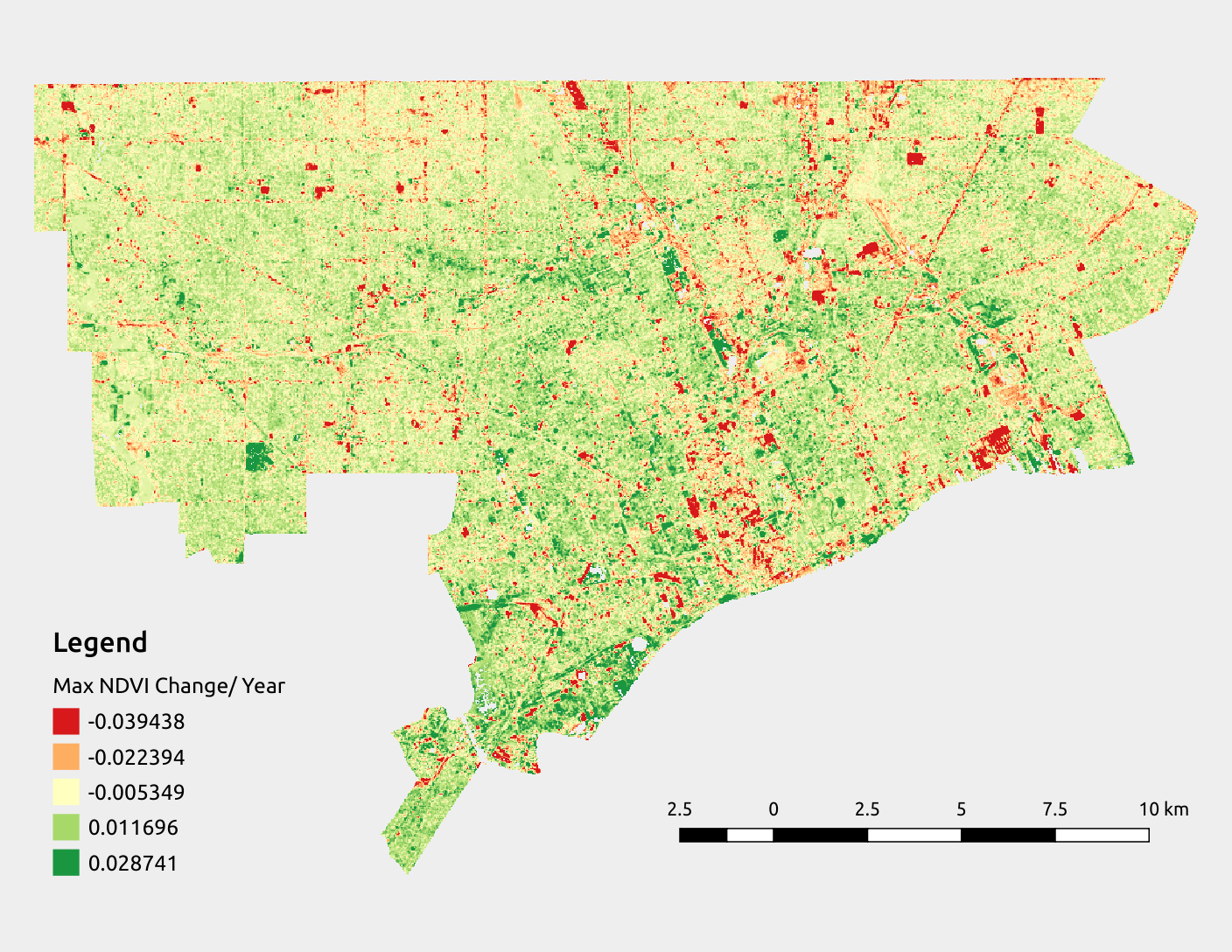
I have a time series of maximum NDVI from 1995 through 2015 (21 images) covering the City of Detroit.
So, to start with, I need to read in each raster file (for each year) and concatenate them together into a single, large, \(N\)-dimensional array, where \(N=21\) for 21 years, in this case.
Strictly speaking, my array ends up being of a size \(N\times Y\times X\) where \(Y,X\) are the number of rows and columns in any given image, respectively (note: each image must have the same number of rows and columns).
Below, I demonstrate this directly; I use the glob library to get a list of files that match a certain pattern: *.tiff.
import glob
import os
import sys
import numpy as np
from osgeo import gdal

# Create a list (generator) of the years, 1995-2015
years_list = range(1995, 2016)
years_array = np.array(years_list)

# Make it a 2-dimensional array to start
years_array = years_array.reshape((1, years_array.shape[0]))

# Get a list of the relevant files; sort in place
ordered_files = glob.glob('*.tiff')
ordered_files.sort()
Note that calling the file list's sort() method is essential: if the files are not in the right order, our regression line won't be fit properly (we will be assigning dependent variables to the wrong independent variable/ wrong year).
Combining Array Data from Multiple Files
Our target array from regression over \(N\) years (files) is a \(P\times N\) array, where \(P = Y\times X\). That is, \(P\) is the product of the number of rows and the number of columns. This array can be thought of as a collection of 1-D subarrays with \(N\) items: the measured outcome (here, maximum NDVI) in each year.
# Iterate through each file, combining them in order as a single array
for i, each_file in enumerate(ordered_files):
    year = years_list[i]

    # Open the file, read in as an array
    ds = gdal.Open(each_file)
    arr = ds.ReadAsArray()
    ds = None
    shp = arr.shape

    # Ravel the array to a 1-D shape
    arr_flat = arr.reshape((shp[0]*shp[1], 1))

    # For the very first array, use it as the base
    if i == 0:
        base_array = arr_flat
        continue # Skip to the next year

    # Stack the arrays from each year
    base_array = np.concatenate((base_array, arr_flat), axis = 1)
Now that we have a suitably shaped array of our dependent variable data, maximum NDVI, we want to generate an array of identical shape of our independent variable, the year.
# Create an array for the X data, or independent variable, i.e., the year
shp = base_array.shape
years_array = np.repeat(years_array, shp[0], axis = 0)\
    .reshape((shp[0], shp[1], 1))
base_array = base_array.reshape((shp[0], shp[1], 1))
Finally, we can combine both our dependent and independent variables into a single \((P\times N\times 2)\) array.
# Now, combine X and Y data
base_array = np.concatenate((years_array, base_array), axis = 2)
Sidebar: Linear Regression in SciPy
Let's take a moment to examine how linear regression works in SciPy (the collection of scientific computing tools that extend from NumPy).
The linear regression function is found as scipy.stats.linregress(); there are at least two ways to specify a linear regression and I opted for the approach that requires a single array argument to the function, e.g.:
from scipy import stats
stats.linregress(x) # e.g., x is a Nx2 array for N regression cases
In this approach, as the SciPy documentation states:
If only x is given (and y=None), then it must be a two-dimensional array where one dimension has length 2. The two sets of measurements are then found by splitting the array along the length-2 dimension.
This is why we created a combined \((P\times N\times 2)\) array; each pixel is then a \((N\times 2)\) subarray that is already set up for the stats.linregress() function.
The last part, since we want to calculate regressions on every one of \(P\) total pixels is to map the stats.linregress() function over all pixels.
We'll define a function to do just this, as below.
The first (zeroth) element in the sequence that is returned is the slope, which is what we want.
def linear_trend(array):
    N = array.shape[0]
    result = [stats.linregress(array[i,...])[0] for i in range(0, N)]
    return result
Calculating Regressions on Subarrays across Multiple Processes
Potential pitfall: It may seem straightforward now to farm out a range of pixels, e.g., \([i,j] \in [0\cdots P]\) for \(P\) total pixels. However, with multiple processes, each process gets a complete copy of the resources required to get the job done. For instance, if you spin up 2 processes asking one to take pixel indices \(0\cdots P/2\) and the other to take pixel indices \(P/2\cdots P\), then each process needs a complete copy of the master (\(P\times N\times 2\)) array. See the issue here? For large rasters, that's a huge duplication of working memory. A better practice is to literally divide the master array into chunks before farming out those pixel (ranges) to each process.
Dividing rectangular arrays in Python based on the number of processes you want to spin up may seem tricky at first.
Below, I use some idiomatic Python to calculate the range of pixel indices each process would get based on P processes (note: here, P is the number of processes, whereas earlier I referred \(P\) as the number of pixels).
N = base_array.shape[0]
P = (NUM_PROCESSES + 1) # Number of breaks (number of partitions + 1)

# Break up the indices into (roughly) equal parts
partitions = list(zip(np.linspace(0, N, P, dtype=int)[:-1],
    np.linspace(0, N, P, dtype=int)[1:]))

# Final range of indices should end +1 past last index for completeness
work = partitions[:-1]
work.append((partitions[-1][0], partitions[-1][1] + 1))
It might be useful if you see what work contains.
In my example, I had 730331 total pixels and I wanted to farm them out, evenly, to 4 processes.
Note that the last range ends on 730332, since the Python range() function does not include the ending number (that is, we want to make sure we count up to, but not including pixel 730332).
>>> work
[(0, 182582), (182582, 365165), (365165, 547748), (547748, 730332)]
Concurrency in Python 3
Finally, to farm out these subarrays to multiple processes, we need to use the ProcessPoolExecutor that ships with Python 3, available in the concurrent.futures module.
Potential pitfall: You might be tempted to use a lambda function in place of the linear_trend() function we defined above, for any similar pixel-wise calcualtion you want to perform.
Because Python multi-process concurrency requires that every object farmed out to multiple processes be "picklable,", you can't use lambda functions. Instead, you must define a global function, as we did, above, with linear_trend().
What does "picklable" mean?
It means that the object can be pickled using Python's pickle library; pickled objects are binary representations of Python state, i.e., of Python data, functions, classes, etc.
Why does each process' state need to be pickled?
I'll let the Python concurrent.futures library answer that directly:
The
ProcessPoolExecutorclass is anExecutorsubclass that uses a pool of processes to execute calls asynchronously.ProcessPoolExecutoruses themultiprocessingmodule, which allows it to side-step the Global Interpreter Lock but also means that only picklable objects can be executed and returned.
If you do need an anonymous or dynamically created function, like a lambda function, you can still use such a pattern with concurrency in Python; you just need to use the partial() function as a wrapper.
The ProcessPoolExecutor creates a context in which we can map a (globally defined, picklable) function over a subset of data.
Because it creates a context, we invoke it using the with statement.
from concurrent.futures import ProcessPoolExecutor

# Split the master array, base_array, into subarrays defined by the
#   starting and ending, i and j, indices
with ProcessPoolExecutor(max_workers = NUM_PROCESSES) as executor:
    result = executor.map(linear_trend, [
        base_array[i:j,...] for i, j in work
    ])
After the processes terminate, their results are stored as a sequence which we can coerce to a list using the list() function.
In our case, in particular, because we split up the \(P\) pixels into 4 sets (for 4 processes), we want to concatenate() them back together as a single array.
regression = list(result)
result = np.concatenate(regression, axis = 0)
And, ultimately, if we want to write the pixel-wise regression out as a raster file, we need to reshape it to a 2-dimensional, \(Y\times X\) raster, for \(Y\) rows and \(X\) columns.
output_array = np.array(result).reshape((num_rows, num_cols))
Performance Metrics
No discussion of concurrency would be complete without an analysis of the performance gain.
If you're not already aware, Python's built-in timeit module is de rigeur for timing Python code; below, I use it to time our pixel-wise regression in both its serial and parallel (multiple-process) forms.
With 4 processes:
$ python -m timeit -s "from my_regression_example import main" -n 3 -r 3 "main('~/Desktop/*.tiff')"
3 loops, best of 3: 46.1 sec per loop
With 1 process (serial):
$ python -m timeit -s "from my_regression_example import main" -n 3 -r 3 "main('~/Desktop/*.tiff')"
3 loops, best of 3: 152 sec per loop
As you can see, with 4 processes we're finishing the work in about one-third of the time as it takes with only one process. You might have expected us to finish in a quarter of the time, but because of the overhead associated with spinning up 4 processes and collecting their results, we never quite get a \(1/P\) reduction in time for \(P\) processes. This speed-up is still quite an achievement, however. No matter how many processes we use, the regression results are, of course, the same; below is the image we created, with colors mapped to regression slope quintiles.
In Summary
By raveling a 2-D raster array into a collection of pixel-level subarrays, we can easily pass any vectorized function over them, allowing us to do far more than regression. With a vectorized function, we can farm out the work to multiple processes to finish our total work faster. In addition, because we split our raster time series up into multiple chunks, the memory required is no more than we need to store the entire raster time series. Keep in mind these two pitfalls that are commonly encountered with multi-processing in Python:
- DON'T use a
lambdafunction as the function to map over the array; instead, use regular, globally defined Python functions, with or withoutfunctools.partial, as needed. - DO chunk up the array into subarrays, passing each process only its respective subarray.
In case my walkthrough above was overwhelming, a general pattern for parallel processing of raster array chunks is presented below.
import glob
import numpy as np
from osgeo import gdal
from concurrent.futures import ProcessPoolExecutor

# Example file list; filenames should have some numeric date/year
ordered_files = glob.glob('*.tiff')
ordered_files.sort()

# A function that maps whatever you want to do over each pixel;
#   needs to be a global function so it can be pickled
def do_something(array):
    N = array.shape[0]
    result = [my_function(array[i,...]) for i in range(0, N)]
    return result

# Iterate through each file, combining them in order as a single array
for i, each_file in enumerate(ordered_files):
    # Open the file, read in as an array
    ds = gdal.Open(each_file)
    arr = ds.ReadAsArray()
    ds = None
    shp = arr.shape
    arr_flat = arr.reshape((shp[0]*shp[1], 1)) # Ravel array to 1-D shape
    if i == 0:
        base_array = arr_flat # The very first array is the base
        continue # Skip to the next year

    # Stack the arrays from each year
    base_array = np.concatenate((base_array, arr_flat), axis = 1)


# Break up the indices into (roughly) equal parts, e.g.,
#   partitions = [(0, 1000), (1000, 2000), ..., (9000, 10001)]
partitions = [...]

# NUM_PROCESSES is however many cores you want to use
with ProcessPoolExecutor(max_workers = NUM_PROCESSES) as executor:
    result = executor.map(linear_trend, [
        base_array[i:j,...] for i, j in partitions
    ])

combined_results = list(result) # List of array chunks...
final = np.concatenate(regression, axis = 0) # ...Now a single array
np.array(final).reshape((num_rows, num_cols)) # ...In the original shape
References
- Breshears, C. 2009. The Art of Concurrency: A Thread Monkey's Guide to Writing Parallel Applications. O'Reilly Media Inc. Sebastopol, CA, U.S.A.
- Beazley, D. 2010. "Understanding the Python GIL." PyCon 2010. Atlanta, Georgia.
- Fortuner, B. 2017. "Intro to Threads and Processes in Python."