Note: This post builds and improves upon an earlier one, where I introduce the Gapminder dataset and use it to explore how diagnostics for fixed effects panel models can be implemented.
Note (July 2019): I have since updated this article to add material on making partial effects plots and to simplify and clarify the example models.
My last post on this topic explored how to implement fixed effects panel models and diagnostic tests for those models in R, specifically because the two libraries I used for this at the time, plm and lfe, in different ways, weren't entirely compatible with R's built-in tools for evaluating linear models.
Here, I want to write a much more general article on fixed effects regression and its implementation in R.
Specifically, I'll write about:
- Use and interpretation of fixed effects (FE) regression models in the context of repeat-measures or longitudinal data;
- How to implement an FE model in R using either the built-in
lm()function or those provided byplmorlfe; - Calculating variance inflation factors (VIF);
- Assessing multi-collinearity among predictor variables before fitting an FE model;
- FE model criticism, including whether or not the assumptions of the linear model are met;
- Calculating and plotting the marginal effect of \(X\) on \(Y\), i.e., partial effects plots.
In this article, I'll be using the Gapminder dataset again; the previous article gives a description of the dataset and its contents.
Use and Interpretation of Fixed Effects Regression
I'm going to focus on fixed effects (FE) regression as it relates to time-series or longitudinal data, specifically, although FE regression is not limited to these kinds of data. In the social sciences, these models are often referred to as "panel" models (as they are applied to a panel study) and so I generally refer to them as "fixed effects panel models" to avoid ambiguity for any specific discipline. Longitudinal data are sometimes referred to as repeat measures, because we have multiple subjects observed over multiple periods, e.g., patients in a clinical trial or households in a study of spending habits throughout the year. You can think of multiple examples where repeat measures are relevant.
As I previously discussed, fixed effects regression originates in the social sciences, in particular in econometrics and, separately, in prospective clinical or social studies:
In these prospective studies, a panel of subjects (e.g., patients, children, families) are observed at multiple times (at least twice) over the study period. The chief premise behind fixed effects panel models is that each observational unit or individual (e.g., a patient) is used as its own control, exploiting powerful estimation techniques that remove the effects of any unobserved, time-invariant heterogeneity
The term "fixed effects" can be confusing, and is contested, particularly in situations where fixed effects can be replaced with random effects. Clark and Linzer (2014) provide a good discussion of the differences and trade-offs between fixed and random effects [1]. Gelman and Hill (2007) or Bolker et al. (2009) also provide good discussions of the differences between fixed and random effects [2,3].
Relevance of Fixed Effects Regression for Causal Inference
Repeat measures are commonly required for a particular type of causal inference. In these studies, the interpretation of a causal effect is that it occurs before or at the same time as the measured outcome (some causal effects appear to be simultaneous with the outcome, such as flipping on a light switch). In fact, FE regression models are often used to establish weak causal inference under certain circumstances; we'll soon see why.
But even where causal inference is not the goal, FE regression models allow us to control for omitted variables. In the context of a regression model, an omitted variable is any variable that explains some variation in our response or dependent variable and co-varies with one or more of the independent variables. It is something that we should be measuring and adding to our regression model because it predicts or explains our dependent variable but also because the relationship between one of our existing independent variables may depend on that omitted variable. For example, if we're interested in measuring the effect of different amounts of a fertilizer on crop yield (i.e., the weight or biomass of the harvested crop) across a set of different crop types, omitted variables might include (if we failed to measure them) the crop type or the type of soil each plant is in. Crop type certainly affects crop yield, as certain crops will have different ranges of yields they can achieve, but also may affect the way that fertilizer drives yields; certain crops may be more or less sensitive to the fertilizer we're using. Soil type, too, will affect yields (without fertilizer, it is the only source of the crop's nutrients) and the properties of the soil may affect how fertilizer is retained and subsequently absorbed by a plant's roots. In our study, failing to account for either crop type or soil type would be a source of omitted variable bias in our study design and in our model.
FE regression models eliminate omitted variable bias with respect to potentially omitted variables that do not change over time. Such time-invariant variables, like crop type or soil type, from our previous example, will be the same for each subject in our model every time it is measured. In a clinical trial, patient sex, eye color, and height (in grown adults) are all examples of time-invariant variables. We'll soon see how the use of subject-level fixed effects control for any and all time-invariant omitted variables. But first, let's appreciate the implications for causal inference.
Let's say we have repeat measures of \(y\), some outcome of interest, and of multiple \(x_i\) or independent variables. We have measured every relevant variable that varies over time and affects \(y\) and/or the relationship between \(y\) and other of the \(x_i\). Furthermore, we have controlled for all sources of time-invariant differences between subjects [1]. That means the only variable(s) that can explain differences in \(y\) are one or more of those time-varying \(x_i\) we have measured. By estimating the effect of \(x_i\) within an individual subject over time, relative to that subject's long-term average conditions, we eliminate the effects of all unobserved, time-invariant heterogeneity between the different subjects. [4]. We can then argue that a change level of any particular \(x_i\)—if it has a sufficient mechanism we can explain—is a likely cause of a corresponding change in \(y\). Much of this depends on the nature of your data, whether or not your proposed treatment variable is reasonable, whether or not you have actually controlled for everything relevant, and, no less important, the reception this type of model will receive from your intended audience (or field of study). In general, causal inference with panel models still requires an assumption of strong exogeneity (simply put: no hidden variables and no feedbacks).
General Specification of Fixed Effects Models
In general, for a sample of subjects indexed \(i\in [0, 1, 2, \dots ]\), where each individual subject can be identified as part of a group, \(j\), of other observations (on the same individual or on multiple other individuals), the outcome for an individual can be modeled as:
In order for this model to be identified, it is essential that the rank of \(i\) be larger than the rank of \(j\), i.e., that there are more individual subjects than there are groups. Otherwise, the \(\alpha_j\) terms would absorb all the degrees of freedom in the model.
Alternative Specifications for Longitudinal Data
Similarly, in a repeat-measures or longitudinal framework, where the "groups" of individuals are time periods, it is essential each individual subject is observed more than once. Obviously, if the number of observations \(N\) was equal to the number of individuals \(i \in M\), we would exhaust the degrees of freedom in our model simply by adding \(M\) intercept terms, \(\alpha_i + ... + \alpha_M\). With as few as two observations \((t \in [1,2])\) of each subject, however, we've doubled the number of observations and the individual intercept terms now correspond to any time-invariant, idiosyncratic change between those two observations.
We can specify our model in two different ways; though very different, they have the same interpretation and will produce the same parameter estimates in a least-squares regression. Compared to the general specification, above, we exchange the index of groups, \(j\), for an index of time periods, \(t\). The first specification is an ordinary least squares (OLS) regression in which a fixed intercept, \(\alpha_i\) is fit for every subject \(i\).
The second specification subtracts the subject-specific mean values of our dependent variable, \(y\), and independent variables, \(X\), from the values at each period of observation, \(t\), for every subject, \(i\).
These two specifications are equivalent because fitting a subject-specific intercept, \(\alpha_i\), effectively reduces the variation in each subject's \(y_i\) and \(X_i\) to variation around its long-term mean. In the first, or fixed-intercept specification, \(\alpha_i\) represents each subject's long-term mean. In the second, or demeaned specification, subtracting the subject-specific mean values of the dependent and independent variables is called centering the data within subjects. This is because the resulting values now have a mean value of zero.
As with everything in statistics, a diverse set of terms have been created to describe the same thing, and the terms used often depend on the lingua franca of a particular discipline. Subtracting the subject-specific means can be variously referred to as centering the data within subjects or time-demeaning the data (subtracting the long-term mean); the centered values themselves can also be referred to as deviations from the (subject-specific) mean.
Interpretation
Setting aside issues of causal inference, how do we interpret a fixed effects regression? Because of the way the data have been transformed (into deviations from subject-specific means), we cannot interpret the coefficients in the same was as for a cross-sectional OLS regression. In the cross-sectional case, we interpret a regression coefficient, \(\beta\), as the change in our dependent variable per unit change in the corresponding independent variable across or between subjects; in a sense, we are estimating the effect of a difference between two subjects, one average in every way, and the other different by one unit in the corresponding independent variable. In a one-way fixed effects regression, because the dependent and independent variables have been transformed to deviations from the subject-specific means, \(\beta\) is instead interpreted as the change in our dependent variable, \(y\), per unit change in the corresponding independent variable, \(x\), within each subject. In this sense, the regression coefficients tell us about the relationship between \(x\) and \(y\) as the subject's \(x\) changes over time. If we accept weak causal inference is justified, the model can be interpreted as: a unit change in \(x\) drives an estimated change in \(y\).
Including Time Period Fixed Effects
This model can be extended further to include both individual fixed effects (as above) and time fixed effects (the "two-ways" model):
Here, \(\mu_t\) is an intercept term specific to the time period of observation; it represents any change over time that affects all observational units in the same way (e.g., the weather or the news in an outpatient study). These effects can also be thought of as "transitory and idiosyncratic forces acting upon [observational] units (i.e., disturbances)" [5].
However, including time period fixed effects changes the interpretation of our model considerably. In the individual fixed effects (only) model, \(\beta\) represented the "within" effect: the effect of a change in \(X_i\) on \(y\) within each individual \(i\). Now, the time period fixed effect functions as an additional grouping in which the data are centered (in our time-demeaning framework, described above). With both time and individual fixed effects, \(\beta\) essentially represents a weighted average between the pooled estimator, \(\beta_{OLS}\) (from an OLS regression without fixed effects), the within estimator from our individual effects model, and a between effect from a model with time fixed effects (only) and no individual effects [6].
As Kropko and Kubinec (2018) write, regarding a similar econometric model to the one we investigate here:
This interpretation will often be difficult to communicate and to understand. The difficulty arises because the interpretation requires two dimensions of comparison, not just one. GDP per capita is negative relative to the country’s over-time average, so we compare a country to itself as it changes over time. But then, by regressing relative democracy on relative GDP per capita for the six countries, the two-way FE coefficient ultimately expresses how one country’s GPD per capita and democracy, relative to itself, compares to another country’s GDP per capita and democracy, relative to itself. If this interpretation does not match the question the model is intended to answer, then we suggest that applied researchers employ methods with interpretations that directly answer the research question.
Implementation in R
Let's load in the Gapminder dataset for the following examples.
Since my previous article, I've discovered there is a gapminder package available for R that makes it easy to load these data into an R session.
library(gapminder)
data(gapminder)
Now let's take a brief look at the data. We're interested in modeling the effect of per-capita GDP on life expectancy. Let's first observed that per-capita GDP has a log-linear relationship with life-expectancy. Taking a base-10 logarithm of right-skewed dollar values is generally good practice, and the plot below shows that doing so here improves the linear relationship with life expectancy.
with(gapminder, plot(log10(gdpPercap), lifeExp,
  main = 'Life Expectancy vs. Log10 Per-Capita GDP'))
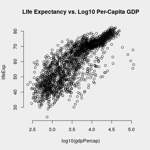
However, for now, we'll model the effect of per-capita GDP without a log transformation because it is simpler.
There are at least three ways to run a fixed effects (FE) regression in R and it's important to be familiar with your options.
With R's Built-in Ordinary Least Squares Estimation
First, it's clear from the first specification above that an FE regression model can be implemented in with R's OLS regression function, lm(), simply by fitting an intercept for each level of a factor that indexes each subject in the data.
m1.ols <- lm(lifeExp ~ country + gdpPercap + pop, data = gapminder)
One disadvantage of this approach becomes clear as soon as you call summary(m1.ols); the subject-specific (here, country-specific) intercepts are reported for 140+ countries in this dataset!
That's a lot to scroll through to get to the coefficients we're actually interested in.
summary(m1.ols)$coefficients[c('gdpPercap', 'pop'),]
              Estimate   Std. Error  t value     Pr(>|t|)
gdpPercap 3.936623e-04 2.973936e-05 13.23708 5.512379e-38
pop       6.196916e-08 4.838246e-09 12.80819 8.746824e-36
We'll interpret these coefficients later. For now, let's convince ourselves that this model produces the same results if we use centered data and no country-level intercepts.
The initial challenge is in centering the data.
I'm going to use a relatively sophisticated tool to do this, simply because I don't know of a reasonable way to do it with base R.
Using the dplyr library's mutate_at() function, we'll calculate a new, centered variable for our dependent variable, lifeExp, and each of the three independent variables.
This new variable has the suffix _dm at the end of its name, which is my abbreviation for "de-meaned" as in the mean has been subtracted from the variable; you can call it whatever you want.
library(dplyr)
gapminder.centered <- gapminder %>%
  group_by(country) %>%
  mutate_at(.vars = vars(year, lifeExp, pop, gdpPercap), .funs = funs('dm' = . - mean(.)))

summary(gapminder.centered$lifeExp_dm)
    Min.  1st Qu.   Median     Mean  3rd Qu.     Max.
-20.8647  -4.2138   0.4733   0.0000   4.5696  17.1973
We can see from the above that the overall mean, across all subjects, is zero.
This is a consequence of the fact that the mean of each subject's measures is zero, so the mean of means is also zero.
To fit the second or demeaned specification of the model using lm(), we plug in each of these centered or demeaned variables.
m2.ols <- lm(lifeExp ~ gdpPercap_dm + pop_dm,
  data = gapminder.centered)
Now, let's compare the coefficients.
cbind(
  coef(m1.ols)[c('gdpPercap', 'pop')],
  coef(m2.ols)[c('gdpPercap_dm', 'pop_dm')]
)
                  [,1]         [,2]
gdpPercap 3.936623e-04 3.936623e-04
pop       6.196916e-08 6.196916e-08
As you can see, the specifications are equivalent. These coefficients are also correct point estimates for the "within" effect of each independent variable on the outcome. However, as we'll discuss, the standard errors are not correct; this OLS model fails to account for the fact that we have repeat measures of each subject. This is a violation of the assumption of independence of errors. With our data, where we have multiple measures for the same country, some elements of the error term, \(\varepsilon\), are not independent. Clustering the standard errors within countries is one solution, which I won't detail here. The more sophisticated approaches to this model discussed below will deliver the correct standard errors.
If you have a very large number of subjects, the lm() function will cease to work for the first specification of our model, with subject-specific intercepts; it simply wasn't designed to fit thousands of intercepts and it will either take a long time to compute or will fail utterly.
This is where the centering approach comes in handy: it is much easier (on the computer) to work with deviations from the mean instead of computing all those subject-specific intercepts.
The plm and lfe libraries, which we'll we discuss next, have no issue with a large number of subjects in your data, and you don't need to think about the two specifications we discussed when you're using those libraries.
With Dedicated Approaches for Mean Deviations
Now let's see how the dedicated packages plm and lfe are used.
I'll give more time to plm because it is my preferred tool, but they both work very well.
Neither of these packages fits intercepts directly, because this doesn't scale well for a large number of subjects.
In cases where there is a very large subject population such an approach, which we tried with OLS, above, could lead to a failure to identify the model.
Instead, these packages have tools to fit FE regression models to data that have been transformed into deviations from subject-specific means or from more complicated deviation measures (in the case of two-ways fixed effects models).
With the lfe package [7], our fixed effects regression of life expectancy on time, per-capita GDP, and total population can be expressed with a syntax similar to the of the popular lme4 and nlme packages.
The felm() function is what we want to use to fit fixed effects models with lfe.
library(lfe)
m1.lfe <- lfe::felm(lifeExp ~ gdpPercap + pop | country,
  data = gapminder)
The | country syntax indicates we wish to fit a fixed intercept for each level of country.
If we compare the coefficient estimates of this model to those of both of our prior OLS models, we'll see that we are indeed fitting exactly the same mean structure in all three approaches.
cbind(
  coef(m1.ols)[c('gdpPercap', 'pop')],
  coef(m2.ols)[c('gdpPercap_dm', 'pop_dm')],
  coef(m1.lfe)
)
If we examine the standard errors, however, we'll see that they are different in the demeaned OLS (or "OLS on mean deviations") model.
std.errs <- cbind(
  summary(m1.ols)$coefficients[c('gdpPercap', 'pop'),2],
  summary(m2.ols)$coefficients[c('gdpPercap_dm', 'pop_dm'),2],
  summary(m1.lfe)$coefficients[,2]
)
colnames(std.errs) <- c('OLS w/ Intercepts', 'OLS on Mean Deviations', 'felm Model')
std.errs
          OLS w/ Intercepts OLS on Mean Deviations   felm Model
gdpPercap      2.973936e-05           6.052637e-05 2.973936e-05
pop            4.838246e-09           9.846931e-09 4.838246e-09
In general, you cannot rely on OLS to deliver the correct standard errors when you have a dependence structure like repeat measures in your data.
In this case, the standard errors for the OLS model with intercepts (first column) are the same as estimated by lfe (third column), because our OLS model does have a dummy variable for each country-specific intercept.
The correction for standard errors, in this case, is straightforward, as the felm() documentation describes:
The standard errors are adjusted for the reduced degrees of freedom coming from the dummies which are implicitly present.
In the second column, we can see that the standard errors for the demeaned OLS model are not correct.
The advantage of lfe (and plm) is that it achieves the computational efficiency of a mean-deviations approach and is also able to estimate the correct standard errors.
Now let's see how plm handles the same model.
In plm, the function we'll use to fit FE regression models is also called plm [8].
Below, the index argument indicates which column has levels corresponding to the subjects, for which individual, subject-level intercepts will be fit implicitly.
m1.plm <- plm(lifeExp ~ gdpPercap + pop, data = gapminder,
  model = 'within', index = c('country'))

summary(m1.plm)
Oneway (individual) effect Within Model

Call:
plm(formula = lifeExp ~ gdpPercap + pop, data = gapminder, model = "within",
    index = c("country"))

Balanced Panel: n = 142, T = 12, N = 1704

Residuals:
     Min.   1st Qu.    Median   3rd Qu.      Max.
-30.23943  -3.25287   0.31427   3.54819  19.85916

Coefficients:
            Estimate Std. Error t-value  Pr(>|t|)
gdpPercap 3.9366e-04 2.9739e-05  13.237 < 2.2e-16 ***
pop       6.1969e-08 4.8382e-09  12.808 < 2.2e-16 ***
---
Signif. codes:  0 ‘***’ 0.001 ‘**’ 0.01 ‘*’ 0.05 ‘.’ 0.1 ‘ ’ 1

Total Sum of Squares:    73973
Residual Sum of Squares: 59768
R-Squared:      0.19203
Adj. R-Squared: 0.11796
F-statistic: 185.378 on 2 and 1560 DF, p-value: < 2.22e-16
If you compare these coefficient estimates to all three previous models, you'll see they're the same.
Other things to note in the summary of plm include:
- We have fit a "Oneway (individual) effect Within Model;" that is, we only fit fixed effects for the individual subjects (countries). In
plm, this is the default. - Our panel data are balanced, that is, every subject (country) has the same number of observations. Here, we have
n = 142countries observed inT = 12time periods (12 different years) for a total number ofN = 1704country-year observations. In general, fixed effects regression models are better understood and more reliable for balanced panels.
The R-squared and adjusted R-squared estimated by plm are for the "full" model, i.e., including the country-level fixed effects.
If you called summary() on our lfe model, you'll see that it reports both the full model R-squared and that of the "projected" model.
The "projected" model R-squared refers to the within R-squared, or the proportion of the variation over time explained by the time-varying covariates.
Diagnostics and Inference in R
Assessing Multicollinearity in Fixed Effects Regression Models
Multicollinearity arises when two or more independent variables are highly correlated with one another. It poses a serious problem for explanatory models of all kinds, including non-parametric and statistical learning approaches, because if the correlation between \(x_i\) and \(x_j\) is large, and both are similarly correlated with the outcome of interest, \(y\), then the model cannot determine which of the two, \(x_i\) or \(x_j\), is explaining the observed variation in \(y\). If multicollinearity exists, linear regression coefficients can be unstable or biased.
A popular way of diagnosing multicollinearity is through the calculation of variance inflation factors (VIFs).
The VIF score indicates the proportion by which the variance of an estimator increases due to the inclusion of a particular covariate.
Calculating VIF scores with fitted models other than those produced by lm() can be tricky (it won't work with plm or lfe models) so the easiest way to calculate VIF scores for a one-way fixed effects regression model is to calculated them over the the corresponding fitted OLS model.
We saw that we could get the time-demeaned panel of the Gapminder data easily enough with dplyr and mutate_at(); below is a second way to do this using plm.
# Assuming we've already fit our plm() model...
design.matrix <- as.data.frame(model.matrix(m1.plm))

# Get the time-demeaned response variable, lifeExp
design.matrix$lifeExp <- plm::Within(
  plm::pdata.frame(gapminder, index = 'country')$lifeExp)

# Fit the OLS model on the demeaned dataset
m3.ols <- lm(lifeExp ~ gdpPercap + pop, data = design.matrix)

# Calculate VIF scores
car::vif(m3.ols)
Here, the VIF scores are all very low, so multicollinearity is not an issue.
Linear Model Assumptions: Homoscedasticity
We can assess homoscedasticity, or constant variance in the residuals, by examining a plot of the model residuals against the fitted values.
Once again, R's fitted() doesn't know how to work with plm model objects, however, we can calculate the fitted values as the difference between the observed values and the model residuals.
par(bg = '#eeeeee')
fitted.values <- as.numeric(gapminder$lifeExp - residuals(m1.plm))
plot(fitted.values, residuals(m1.plm),
  bty = 'n', xlab = 'Fitted Values', ylab = 'Residuals',
  main = 'Residuals vs. Fitted')
abline(h = 0, col = 'red', lty = 'dashed')
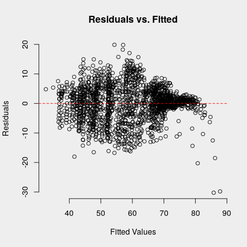
There certainly seems to be some heteroscedasticity present, particularly in the presence of relatively large, negative residuals or high fitted values. Studentized residuals are one way of assessing the magnitude of residual in standardized units [8]. To get studentized residuals, we first have to derive hat matrix (or "projection matrix") from our linear model. This is the matrix given by the linear transformation by which we obtained the estimated coefficients for our model, \(\beta\).
Where \(X\) is the design matrix (matrix of explanatory variables) and \(y\) is the vector of our observed response values.
The hat (or projection) matrix is denoted by \(P\).
The diagonal of this \(N\times N\) matrix (diag(P) in R) contains the leverages for each observation point.
In R, we use matrix multiplication and the solve() function (to obtain the inverse of a matrix).
# Calculate projection matrix
X <- model.matrix(m1.plm)
P <- X %*% solve(t(X) %*% X) %*% t(X)

# Internally studentized residuals
sigma.sq <- (1 / m1.plm$df.residual) * sum(residuals(m1.plm)^2)
student.resids <- residuals(m1.plm) / (sigma.sq * (1 - diag(P)))

plot(fitted.values, student.resids, bty = 'n',
  xlab = 'Life Expectancy (Fitted Values)', ylab = 'Residuals',
  main = 'Studentized Model Residuals v. Fitted Values')
abline(h = 0, lty = 'dashed', col = 'red')
The apparent (perceived) distribution of the residuals is the same, but the y-axis now shows standardized units.
Checking for Influential Observations
Sometimes, a linear relationship can be dominated by a small number of highly influential observations. One way this can happen is if the domain of a certain \(X_i\), say, per-capita GDP, is relatively small for most observations (e.g., most countries in a given sample have per-capita GDP in the range of $1,000-2,000) but there are a few countries which have very high per-capita GDP, say, around $5,000. The relationship between per-capita GDP and some outcome like life expectancy, for the group of countries with per-capita GDP in the range $1,000-2,000 might be nothing: the slightly wealthier countries don't have significantly higher life expectancies. However, if the very wealthy countries, with per-capita GDP around $5,000, have considerably higher life expectancy, then a positive relationship will be found between the two even though, if the very wealthy countries were removed, no such relationship would be found.
We can calculate the leverage that a particular observation (country) exerts on a linear relationship; it is like a measure of how sensitive that relationship is to a particular observation.
With the faraway package, we can draw a half-normal plot which sorts the observations by their leverage.
The labs argument will ensure that they are labeled by their row index, and nlab indicates how many points to label (to avoid visual clutter), starting with the most highly influential observation.
X <- model.matrix(m1.plm)
P = X %*% solve(t(X) %*% X) %*% t(X)

require(faraway)
# Create `labs` (labels) for 1 through 1704 observations
halfnorm(diag(P), labs = 1:1704, ylab = 'Leverages', nlab = 1)
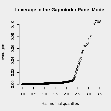
It does seem like there are a few observations that may be driving the relationship. If we index the Gapminder data, we see that India's survey in 2007 is the most influential.
gapminder[708,]
# A tibble: 1 x 6
  country continent  year lifeExp        pop gdpPercap
  <fct>   <fct>     <int>   <dbl>      <int>     <dbl>
1 India   Asia       2007    64.7 1110396331     2452.
It's helpful to look at the data in all years to understand why. It seems that India's per-capita GDP rose quite fast from 2002 to 2007, along with its life expectancy. If we think India's change in this period is an outlier, we may want to remove India from our panel dataset and run the model again.
gapminder[gapminder$country == 'India',]
# A tibble: 12 x 6
   country continent  year lifeExp        pop gdpPercap
   <fct>   <fct>     <int>   <dbl>      <int>     <dbl>
 1 India   Asia       1952    37.4  372000000      547.
 2 India   Asia       1957    40.2  409000000      590.
 3 India   Asia       1962    43.6  454000000      658.
 4 India   Asia       1967    47.2  506000000      701.
 5 India   Asia       1972    50.7  567000000      724.
 6 India   Asia       1977    54.2  634000000      813.
 7 India   Asia       1982    56.6  708000000      856.
 8 India   Asia       1987    58.6  788000000      977.
 9 India   Asia       1992    60.2  872000000     1164.
10 India   Asia       1997    61.8  959000000     1459.
11 India   Asia       2002    62.9 1034172547     1747.
12 India   Asia       2007    64.7 1110396331     2452.
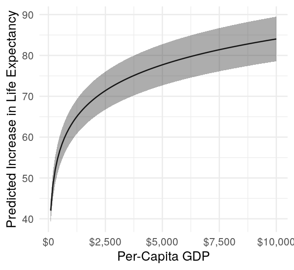
Partial Effects Plots
What is the marginal effect of \(X\) on \(Y\)? This can be read directly from the summary() table, but sometimes it is nicer to visualize as a plot. Such plots are often referred to as partial effects plots [9].
First, let's switch to a different model of life expectancy. We recognized earlier that per-capita GDP really has a log-linear relationship with life expectancy.
m2.plm <- plm(lifeExp ~ I(log10(gdpPercap)) + pop, data = gapminder,
  model = 'within', index = c('country'))
summary(m2.plm)
...
Coefficients:
                      Estimate Std. Error t-value  Pr(>|t|)
I(log10(gdpPercap)) 2.1008e+01 6.9613e-01 30.1779 < 2.2e-16 ***
pop                 3.2964e-08 4.1982e-09  7.8521 7.553e-15 ***
---
Signif. codes:  0 ‘***’ 0.001 ‘**’ 0.01 ‘*’ 0.05 ‘.’ 0.1 ‘ ’ 1

Total Sum of Squares:    73973
Residual Sum of Squares: 41976
R-Squared:      0.43255
Adj. R-Squared: 0.38053
F-statistic: 594.56 on 2 and 1560 DF, p-value: < 2.22e-16
This model fits much better, which is obvious when we look at plots of the raw data but also when we examine how the goodness-of-fit score (R-squared) has changed.
First, let's decide what range of predictor values we want to test. We're interested in the effect of per-capita GDP on life expectancy. Let's look at rising per-capita GDP; this will be our parameter sweep. Recall that in our subject-centered model, these values are deviations from the mean, i.e., positive values represent per-capita GDP above the mean for the average subject.
# Create a test matrix
gdpPercap.sweep <- log10(seq(100, 10e3, 1e2)) # A parameter sweep of per-capita GDP change
Next, we want to get an empty design or model matrix. By "empty" I mean that the values in all columns are zero. This is because, in our subject-centered model, the mean value of any variable is going to be zero (because we subtracted the mean within each subject).
# Get the columns in the same order
new.X <- model.frame(m2.plm)
new.X <- new.X[,names(coef(m2.plm))]
stopifnot(colnames(new.X) == names(coef(m2.fe)))

# Get a short representation of design matrix
test.X <- colMeans(new.X)
test.X[1:length(test.X)] <- 0 # Mean value for subject-centered data is always zero)

# Fill out an empty test matrix
test.X <- matrix(rep(test.X, each = length(gdpPercap.sweep)), nrow = length(gdpPercap.sweep))
Then, we need to insert our parameter sweep into this empty design matrix. All other variables will have zero everywhere, but the variable we're interested in (per-capita GDP) needs to meaningfully change so we can visualize its effect on the outcome (life expectancy).
# Insert the parameter sweep
test.X[,which(colnames(new.X) == 'I(log10(gdpPercap))')] <- gdpPercap.sweep
Finally, we're ready to calculate the partial effect and the confidence band. The partial effect is the predicted value of \(Y\) (life expectancy) for a given value of \(X\) (per-capita GDP). We want to visualize the uncertainty around this prediction, so we'll also calculate the standard error of the prediction and use this to derive a 95% confidence interval around the prediction.
level <- 0.95 # For a 95% confidence interval

# Get the covariance matrix of the predictions
vcov.prediction <- test.X %*% vcov(m2.plm) %*% t(test.X)

# The standard error of the prediction is then on the diagonal
se.prediction <- sqrt(diag(vcov.prediction))

# Get the predicted value by multiplying the design matrix
#   against our coefficient estimates
predicted <- (test.X %*% coef(m2.plm))

# Calculate the t-statistic corresponding to a 95% confidence level and
#   the appropriate num. of degrees of freedom
t.stat <- qt(1 - (1 - 0.95)/2, m2.plm$df.residual)

# Calculate the lower and upper bounds of the confidence interval
lower.bound <- as.numeric(predicted - t.stat * se.prediction)
upper.bound <- as.numeric(predicted + t.stat * se.prediction)
We can quickly verify we're getting reasonable results.
head(cbind(lower.bound, predicted, upper.bound))
     lower.bound          upper.bound
[1,]    39.28448 42.01537    44.74627
[2,]    45.19739 48.33932    51.48125
[3,]    48.65621 52.03859    55.42096
[4,]    51.11029 54.66326    58.21623
[5,]    53.01382 56.69912    60.38441
[6,]    54.56912 58.36253    62.15595
Recall that the first row corresponds to a $100 increase in per-capita GDP within a given country; our model predicts that the life expectancy would increase by about 42 years for such an increase in per-capita GDP! This can also be derived from the slope of the gdpPercap coefficient:
coef(m2.plm)[1]
I(log10(gdpPercap))
           21.00769
A 2-unit increase in the log of per-capita GDP corresponds to a $100 increase, so an increase of life expectancy of \(2\times 21 = 42\) years is expected. From the 95% confidence interval we just calculated, we can see that a better estimate of the effect could be given as a range between 39.3 and 44.7 years.
This seems really large; likely our model is too simple. Our model controls for all time-invariant confounding factors, but there are likely other factors that change with time (i.e., not time-invariant) that we are missing. Thus, even though our current model is robust against heterogeneity, the results are likely still biased. Our results could also be affected by mixing very poor and very wealthy countries together; small increases in per-capita GDP may indeed have outsized effects in very poor countries, but certainly not in wealthy nations.
Without recourse to greater model realism, we can at least make the partial effects plot using ggplot2. We note that larger and larger increases in per-capita GDP do have a diminishing effect on life expectancy, which is reasonable.
library(ggplot2)
library(scales)
df <- data.frame(gdpPercap = gdpPercap.sweep,
  prediction = predicted,
  lower = lower.bound,
  upper = upper.bound)
ggplot(df, mapping = aes(x = 10^gdpPercap, y = prediction)) +
  geom_line() +
  geom_ribbon(mapping = aes(ymin = lower, ymax = upper), alpha = 0.4) +
  scale_x_continuous(labels = dollar) +
  labs(x = 'Per-Capita GDP', y = 'Predicted Increase in Life Expectancy') +
  theme_minimal()
References
- Clark, T. S., & Linzer, D. A. (2014). Should I Use Fixed or Random Effects? Political Science Research and Methods, 3(02), 399–408.
- Gelman, A., and J. Hill. 2007. Data Analysis Using Regression and Multilevel/Hierarchical Models. New York, New York, USA: Cambridge University Press.
- Bolker, B. M., M. E. Brooks, C. J. Clark, S. W. Geange, J. R. Poulsen, M. H. H. Stevens, and J. S. S. White. 2009. Generalized linear mixed models: a practical guide for ecology and evolution. Trends in Ecology and Evolution 24(3):127–135.
- Allison, P. D. 2009. Fixed Effects Regression Models ed. T. F. Liao. Thousand Oaks, California, U.S.A.: SAGE.
- Halaby, C. N. 2004. Panel Models in Sociological Research: Theory into Practice. Annual Review of Sociology 30(1):507–544.
- Kropko, J., & Kubinec, R. (2018). Why the Two-Way Fixed Effects Model Is Difficult to Interpret, and What to Do About It. SSRN, 1–27.
- Gaure, S. (2013). lfe: Linear Group Fixed Effects. The R Journal, 5(2), 104–117. Retrieved from http://journal.r-project.org/archive/2013-2/gaure.pdf
- Croissant, Y., & Millo, G. (2008). Panel data econometrics in R: The plm package. Journal of Statistical Software, 27(2), 1–43.
- Faraway, J. J. (n.d.). Linear Models with R (2nd ed.). Boca Raton, U.S.A.; London, England; New York, U.S.A.: Chapman & Hall/CRC Texts in Statistical Science.