The Landat Surface Reflectance (SR) product sometimes contains saturation in one or more bands (a value of 16,000 reflectance units or 160% reflectance). Presumably, these correspond to saturation at the detector; the same kind of saturation that is likely to occur over clouds or snow-covered areas. Such clouds and snow can be masked out with a provided masking layer (like CFMask) but there are other land covers like bright soil, deserts, water, and impervious surface that can saturate one or more bands (e.g., Asner et al. 2010; Rashed et al. 2001).
In the summer ("leaf-on" season), we can be confident that, in most areas, snow simply isn't a possible land cover type. Urban areas are full of bright targets, however, and it seems that almost every surface reflectance image contains a few saturated pixels not due to clouds or snow. The saturation value (16,000 for Landsat SR; 20,000 for Landsat top-of-atmosphere reflectance) may not be present in all bands—some targets are only thermally bright while others can produce spectral reflections in the optical bands (e.g., sun glint). Thus, it seems that these bright targets aren't always masked by the included quality assurance (QA) layer; there is still spectral reflectance information in the bands that aren't saturated.
Saturated pixels are easily masked; I'll provide some sample Python code that shows how. But can saturated pixels be ignored or are they a problem for certain types of analyses? I'm currently in the midst of a study of urban reflectance in Southeast Michigan, using spectral mixture analysis to estimate the fractional abundance of certain land cover types. To improve the abundance estimates (by improving the signal-to-noise ratio of the input) and to reduce throughput, I use a minimum noise fraction (MNF) transformation, akin to a principal components rotation that projects the Landsat TM/ETM+ reflectance to an orthogonal basis. Although I had masked these saturated pixels from the start I began to wonder what the difference would be if I had left them in.
The example I present here is for a Landsat 7 ETM+ SR image that has been clipped to Oakland County, Michigan (from within WRS-2 row 20, path 30). The Landsat 7 ETM+ image was captured in July 1999 (ordinal day 196); the image identifier is LE70200301999196EDC00. The original SR image had the QA mask, provided by the USGS, applied to the image in both cases; where saturation was masked and where it was not.
Visualizing Saturation in the Mixing Space
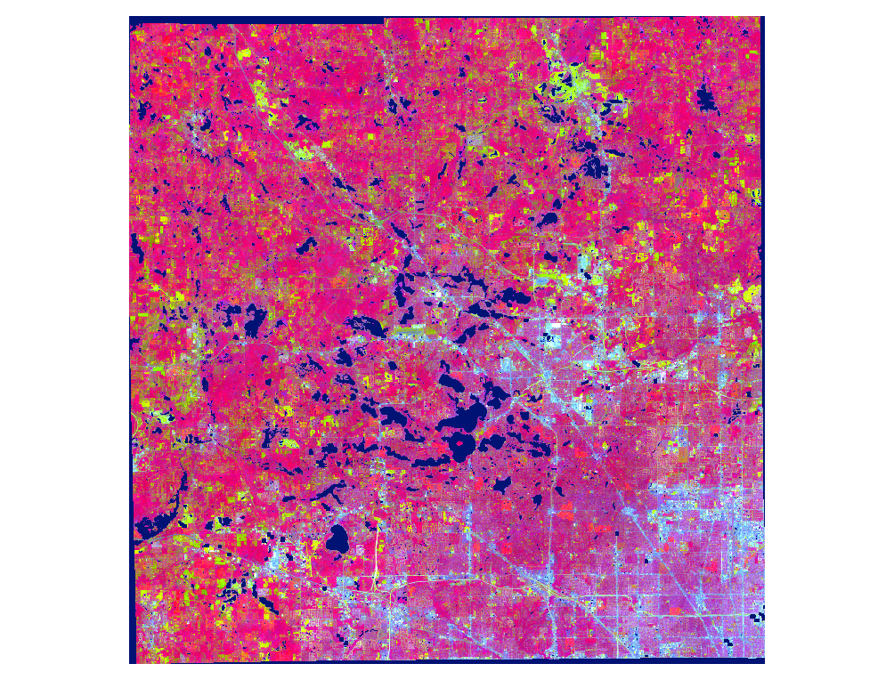
If saturation persists prior to the transformation, the transformed values are scaled differently than when they are first removed. This can be seen "heads-up" in a GIS by toggling between layers: The MNF-transformed image with saturated values (below, left) and the one without (below, right).

It can also be seen in the histograms (left, with saturation; right, without).
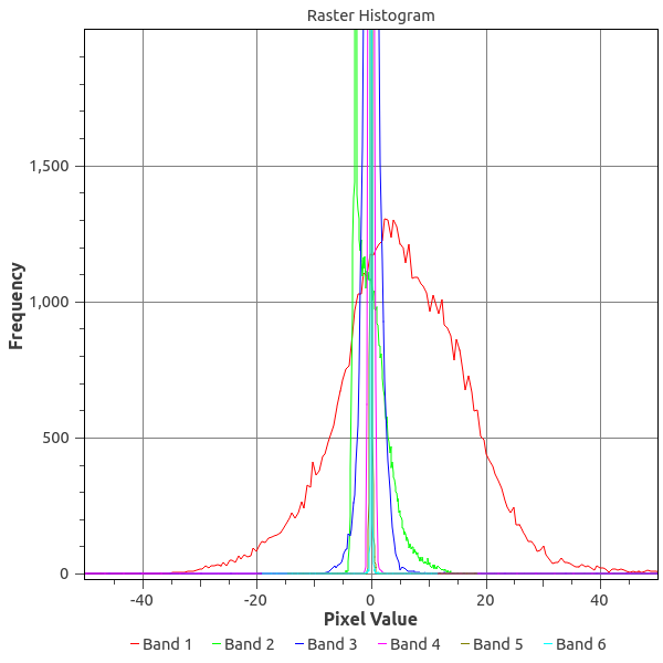
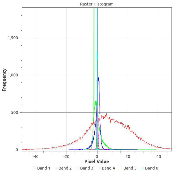
It's interesting to note that the raster image with saturation shows much brighter soil/ cropland areas (yellow in the image) than in the raster image where saturated values were masked. This would seem to suggest that leaving the fully (and partially) saturated pixels in place prior to transformation could improve the accuracy of the abundance estimation. The change in the histograms is not so easy to interpret, however.
Another way of visualizing the difference between these two images is to examine their feature spaces. Below is an example of the mixing space of the image where saturated pixels were not masked; a 2D slice of the feature space showing the first three MNF components. These are the three components with the highest signal-to-noise ratio (SNR) where the SNR of the first component is greater than that of the second, and so on. We see that there are several pixels in this mixing space that are far-flung from the main volume.
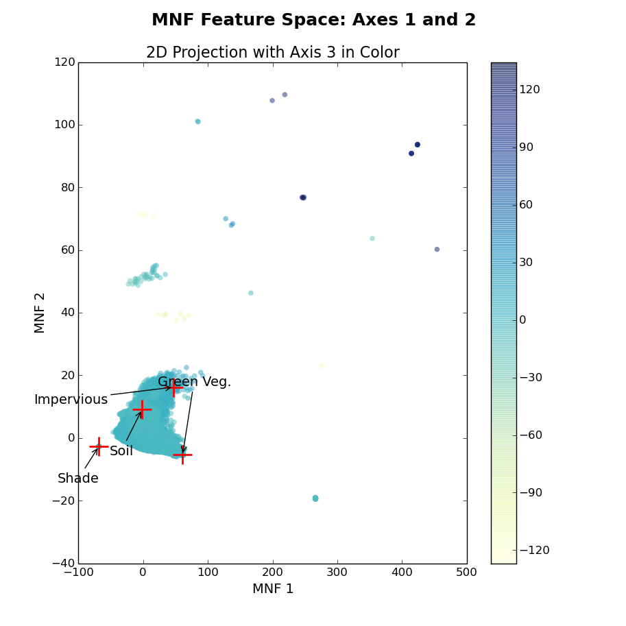
If you're unaccustomed to looking at images like the one above, take my word for it: This looks wrong. Or don't take my word for it; see Tompkins et al. (1997), Wu and Murray (2003) or Small (2004) for examples of mixture spaces. But then what does the feature space look like for the transformed image where saturation was masked? Below, right, is the feature space for that image. On the left, again, is the image where saturation persists, yet I've "zoomed in" to the main mixture volume to facilitate a fair comparison between these images.
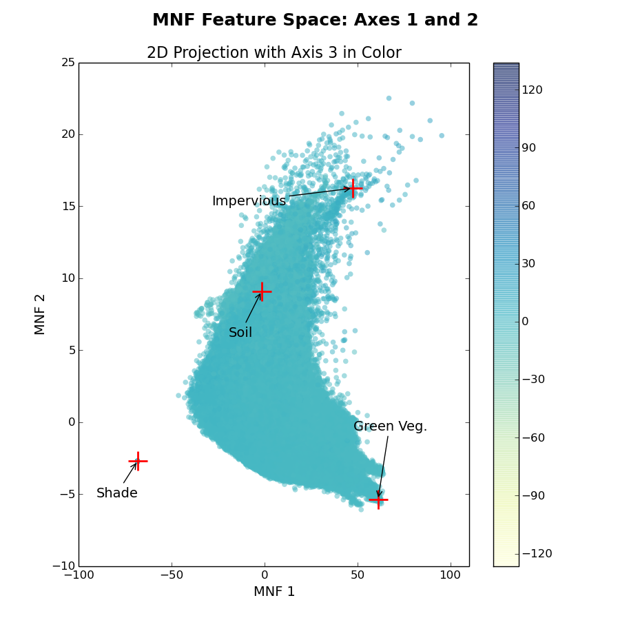
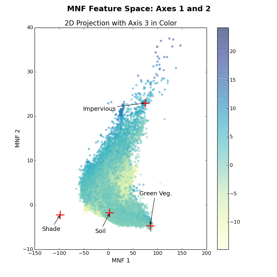
Now these mixing spaces look like what we see in the literature: They should be well-defined convex volumes. They should resemble a ternary diagram. We can see that in the left-hand plot (with saturation), the third MNF component (represented in color) has such a wide range of values that the mixture volume is all one color; there are extreme values in this componenent that are not in view. Those must be the pixels we intially saw scattered throughout the space. The right-hand plot (without saturation) seems properly scaled. Note that I've indicated the locations of pixels with known ground cover types in both plots.
Masking Saturation in Python with GDAL and NumPy
How did I mask the saturated values, by the way? It can be tricky when one or more but not all of the bands are saturated at a given pixel. Below is a Python function, utilizing GDAL and NumPy, that demonstrates how this might be done.
from osgeo import gdal
import numpy as np

def mask_saturation(rast, nodata=-9999):
    '''
    Masks out saturated values (surface reflectances of 16000). Arguments:
        rast    A gdal.Dataset or NumPy array
        nodata  The NoData value; defaults to -9999.
    '''
    # Can accept either a gdal.Dataset or numpy.array instance
    if not isinstance(rast, np.ndarray):
        rast = rast.ReadAsArray()

    # Create a baseline "nothing is saturated in any band" raster
    mask = np.empty((1, rast.shape[1], rast.shape[2]))
    mask.fill(False)

    # Update the mask for saturation in any band
    for i in range(rast.shape[0]):
        np.logical_or(mask,
            np.in1d(rast[i,...].ravel(), (16000,)).reshape(rast[i,...].shape),
            out=mask)

    # Repeat the NoData value across the bands
    np.place(rast, mask.repeat(rast.shape[0], axis=0), (nodata,))
    return rast
What Leads to Better Estimates?
The differences I've shown above are interesting but what actually leads to more accurate estimation of fractional land cover abundances in spectral mixture analysis? I performed a linear spectral mixture analysis on the MNF-transformed images using the same four (4) image endmembers: Impervious surface, Green vegetation, Soil, and Shade. The shade endmember is actually photometric shade: zero reflectance in all bands. Both water and "NoData" pixels are masked to this value as the linear algebra libraries used cannot work with "NoData" values and masked arrays in NumPy have serious performance drawbacks.
One measure of the "fit" between our abundance estimates and reality is to compare the observed to predicted Landsat ETM+ reflectance, where predicted reflectance is computed by a forward model using the endmember spectra and their estimated fractional abundance in a given pixel. It is standard practice (e.g., Rashed et al. 2003; Wu and Murray, 2003) to calculate this "fit" at the root mean squared error (RMSE) between the observed reflectance and the predicted reflectance. Powell et al. (2007) presents a formula for the RMSE of a pixel \(i\) that is normalized by the number of endmembers, \(M\):
I then normalized the sum of the RMSE values across a large, random subset of the pixels (for performance considerations) by the range in reflectances, \(r\):
As the minimum reflectance is always zero (given the presence of shade), \(r_{min} \equiv 0\). The abundance images are each compared to their respective, original Landsat ETM+ image; with or without saturated pixels masked out, as the case may be.
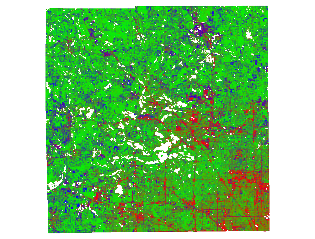
Percent RMSE was calculated for both abundance estimates (with and without saturation) where abundance was estimated two different ways each time: Through a non-negative least squares (NNLS) estimation and through a fully-constrained least squares (FCLS) estimation. With FCLS, abundance estimates are constrained to be both non-negative and on the interval \([0,1]\). With NNLS, the second constraint is dropped. The final abundance images, with or without saturated pixels, look very similar. The FCLS image from the estimate without saturated pixels is below. Impervious surface is mapped to red, vegetation to green, and soil to blue; each pixel's abundance estimates were re-summed to one after shade was subtracted.
Results from the validation are in the table below.
=============================
Saturation?   Approach  %RMSE
-----------   --------  -----
Yes           NNLS       7.9%
No            NNLS       9.2%
Yes           FCLS       1.2%
No            FCLS       3.2%
=============================
It would seem that leaving saturated pixels unmasked results in improved modeling of the ETM+ reflectance. This is only a first approximation of the accuracy, however; we don't really care about the modeled reflectance. The true validation is in comparing the abundance estimates to ground data.
Validation of Abundance Estimates
Shade and soil were subtracted from the abundance images before validation against manually interpreted land cover from aerial photographs in 90-meter windows centered on random sampling points. 169 sample points were located in Oakland County and the coefficient of determination \(\left( R^2 \right)\), RMSE, and mean absolute error (MAE) were calculated for each of the abundance images.
Without saturation:
============================
N     R^2     MAE     RMSE
---   ------  ------  ------
169   0.4742  0.1534  0.1998
============================
With saturated pixels retained:
============================
N     R^2     MAE     RMSE
---   ------  ------  ------
169   0.4360  0.1557  0.2069
============================
Conclusion
Despite the better performance in the forward model, the image in which saturated pixels were retained provided worse estimates than the image in which they were masked. Removing the saturated pixels seems to improve the accuracy of abundance estimates. The magnitude of the improvement is small and we cannot be sure, from this test case alone, that the improvement is not simply a coincidence&emdash;that is, while removing these saturated pixels improved the results in this case, it may be that the saturated pixels in place in another image conspire to produce equal or better results to estimates where they are removed.
However, given the topology of the feature space, the most likely explanation for this marginal improvement in accuracy is the removal of saturated pixels. And perhaps the most important reason for masking saturated pixels is that it makes interpretation of the mixing space much easier.
References
- Asner, G. P., and K. Heidebrecht. 2010. Spectral unmixing of vegetation, soil and dry carbon cover in arid regions: Comparing multispectral and hyperspectral observations. International Journal of Remote Sensing 23 (19):3939–3958.
- Rashed, T., J. R. Weeks, M. S. Gadalla, and A. G. Hill. 2001. Revealing the Anatomy of Cities through Spectral Mixture Analysis of Multispectral Satellite Imagery: A Case Study of the Greater Cairo Region, Egypt. Geocarto International 16 (4):7–18.
- Rashed, T., J. R. Weeks, D. A. Roberts, J. Rogan, and R. L. Powell. 2003. Measuring the Physical Composition of Urban Morphology Using Multiple Endmember Spectral Mixture Models. Photogrammetric Engineering & Remote Sensing 69 (9):1011–1020.
- Green, A. A., M. Berman, P. Switzer, and M. D. Craig. 1988. A transformation for ordering multispectral data in terms of image quality with implications for noise removal. IEEE Transactions on Geoscience and Remote Sensing 26 (1):65–74.
- Tompkins, S., J. F. Mustard, C. M. Pieters, and D. W. Forsyth. 1997. Optimization of Endmembers for Spectral Mixture Analysis. Remote Sensing of Environment 59 (3):472–189.
- Wu, C., and A. T. Murray. 2003. Estimating impervious surface distribution by spectral mixture analysis. Remote Sensing of Environment 84 (4):493–505.
- Small, C. 2004. The Landsat ETM+ spectral mixing space. Remote Sensing of Environment 93 (1-2):1–17.
- Powell, R. L., D. A. Roberts, P. E. Dennison, and L. L. Hess. 2007. Sub-pixel mapping of urban land cover using multiple endmember spectral mixture analysis: Manaus, Brazil. Remote Sensing of Environment 106 (2):253–267.